Sequential Monte Carlo Samplers
$\newcommand{\ystar}{y^{*}} \newcommand{\Ycal}{\mathcal{Y}} \newcommand{\isample}{^{(i)}} \newcommand{\kernel}{p_{\epsilon}(\ystar \mid y)} \newcommand{\tkernel}{\tilde{p}_{\epsilon}(\ystar \mid y)} \newcommand{\jointABCpost}{p_{\epsilon}(\theta, y \mid \ystar)} \newcommand{\like}{p(y \mid \theta)} \newcommand{\prior}{p(\theta)} \newcommand{\truepost}{p(\theta \mid \ystar)} \newcommand{\ABCpost}{p_{\epsilon}(\theta \mid \ystar)} \newcommand{\ABClike}{p_{\epsilon}(\ystar \mid \theta)} \newcommand{\kerneltilde}{\tilde{p}_{\epsilon}(\ystar \mid y)} \newcommand{\zkernel}{Z_{\epsilon}} \newcommand{\truelike}{p(\ystar \mid \theta)} \newcommand{\Ebb}{\mathbb{E}}$
Problem Set-Up
This is all taken from Sequential Monte Carlo samplers. We have a collection of target distributions $$ \pi_n(x) = \frac{\gamma_n(x)}{Z_n} $$ and we would like to sample from them sequentially in order to approximate expectations.
Importance Sampling
We write target expectations using the Importance Sampling (IS) trick for a proposal density $\eta_n$ $$ \Ebb_{\pi_n}[\phi] = \int_E \phi(x) \pi_n(x) dx = \frac{1}{Z_n} \int_E \phi(x) \gamma_n(x) dx = \frac{1}{Z_n} \int_E \phi(x) w_n(x) \eta_n(x) dx $$ $$ Z_n = \int_E \gamma_n(x) dx = \int_E w_n(x) \eta_n(x) dx $$ where we have defined importance weights as $$ w_n(x) = \frac{\gamma_n(x)}{\eta_n(x)} $$ Therefore importance sampling uses the following particle approximation $$ \eta_n^N(dx) = \frac{1}{N} \sum_{i=1}^N \delta_{X_n^{(i)}}(dx) $$ Plugging this into the two expressions above we obtain \begin{align} \Ebb_{\pi_n}[\phi] = \frac{\Ebb_{\eta_n}[\phi w_n]}{\Ebb_{\eta_n}[w_n]} \approx \frac{\Ebb_{\eta_n^N}[\phi w_n]}{\Ebb_{\eta_n^N}[w_n]} = \frac{\sum_{i=1}^N \phi(X_n^{(i)}) w_n(X_n^{(i)})}{\sum_{i=1}^N w_n(X_n^{(i)})} = \sum_{i=1}^N \phi(X_n^{(i)}) W_n(X_n^{(i)}) \end{align} where we have defined the normalized importance weights $$ W_n(X_n^{(i)}) = \frac{w_n(X_n^{(i)})}{\sum_{j=1}^N w_n(X_n^{(j)})} $$
Sequential Importance Sampling
In importance sampling, for each different target $\pi_n$ we would sample the particles afresh from $\eta_n$. This assumes that we can sample from $\eta_n\approx \pi_n$ and that we can evaluate $\eta_n$ in order to evaluate the unnormalized IS weights $$ w_n(x) = \frac{\gamma_n(x)}{\eta_n(x)} $$ In Sequential Importance Sampling (SIS) we start using IS at $n=1$ but then we build $\eta_n$ from the previous iteration. Specifically we do this:
- At time $n=1$ our target is $\pi_1$ and we use an IS proposal $\eta_1$ which we choose to approximate well $\pi_1$ (often we choose $\eta_1 = \pi_1$). This means we sample particles $X_1^{(1:N)}$ from $\eta_1$ and then compute the IS unnormalized weights $$ w_1(X_1^{(i)}) = \frac{\gamma_1(X_1^{(i)})}{\eta_1(X_1^{(i)})} $$
- Suppose that at time $n-1$ we had a set of particles $\{X_{n-1}^{(i)}\}$ sampled from $\eta_{n-1}$. Our target at time $n$ is $\pi_n$. In order to propose a new set of particles we use a Markov Kernel $K_n(x’ \mid x)$. We call the resulting distribution $\eta_n$. Notice that this distribution can be found using the property that a kernel $K_n$ operates on measures on the left $$ \eta_n = \eta_{n-1} K_n \implies \eta_n(x’) = \int_E \eta_{n-1}(x) K_n(x’ \mid x) dx $$ Once we have sampled from the kernel to move the particles forward $X_n^{(i)} \sim K_n(\cdot \mid X_{n-1}^{(i)})$, we need to compute the weights to account for the discrepancy of sampling from $\eta_n$ rather than $\pi_n$ $$ w_n(X_n^{(i)}) = \frac{\gamma_n(X_n^{(i)})}{\eta_n(X_n^{(i)})} $$ However notice we can only do this if we can evaluate $\eta_n$.
In general, we cannot evaluate $\eta_n$ because it is defined in terms of an integral with respect to $x_{1:n-1}$. Indeed consider $\eta_3$
\begin{align} \eta_3(x_3) &= \int_E \eta_2(x_2) K_3(x_3 \mid x_2) dx_2 \newline &= \int_E \left[\int_E \eta_1(x_1) K_2(x_2 \mid x_1) dx_1\right] K_3(x_3 \mid x_2) dx_2 \newline &= \int_{E^2} \eta_1(x_1) K_3(x_3 \mid x_2) K_2(x_2 \mid x_1) dx_1 dx_2 \end{align}
In general $\eta_n$ will be $$ \eta_n(x_n) = \int_{E^{n-1}} \eta_1(x_1) \prod_{k=1}^{n} K_k(x_k \mid x_{k-1}) d x_{1:k-1} $$ which is clearly intractable.
SMC sampler
Since the problem is integration with respect to $x_{1:k-1}$ we “open up” the integral and instead consider its integrand. Rather than considering $\eta_n(x_n)$ which proposes a new set of particles $\{X_n^{(i)}\}$ from $\{X_{n-1}^{(i)}\}$ we consider the proposal distribution $\eta_n(x_{1:n})$ defined as $$ \eta_n(x_{1:n}) = \eta_1(x_1) \prod_{k=2}^{n} K_k(x_k \mid x_{k-1}) $$ We would now like to perform importance sampling. To do this, we need to extend the target from $\pi_n(x_n)$ to $\widetilde{\pi}_n(x_{1:n})$. We do this by introducing backward kernels $L_{n-1}(x_{n-1} \mid x_n)$ $$ \widetilde{\pi}_n(x_{1:n}) = \frac{1}{Z_n} \widetilde{\gamma}_n(x_{1:n}) = \frac{1}{Z_n} \gamma_n(x_n) \prod_{k=1}^{n-1} L_k(x_{k} \mid x_{k+1}) $$ The IS weights would then become \begin{align} w_n(x_{1:n}) &= \frac{\widetilde{\gamma}_n(x_{1:n})}{\eta_n(x_{1:n})} \newline &= \frac{\gamma_n(x_n) \prod_{k=1}^{n-1} L_k(x_{k} \mid x_{k+1})}{\eta_1(x_1) \prod_{k=2}^{n} K_k(x_k \mid x_{k-1})} \newline &= \frac{\gamma_n(x_n) L_{n-1}(x_{n-1} \mid x_n) L_{n-2}(x_{n-2} \mid x_{n-1}) \cdots L_1(x_1 \mid x_2)}{\eta_1(x_1) K_n(x_n \mid x_{n-1}) K_{n-1}(x_{n-1} \mid x_{n-2}) \cdots K_2(x_2 \mid x_1)} \newline &= \frac{\gamma_n(x_n) L_{n-1}(x_{n-1} \mid x_n)}{\gamma_{n-1}(x_{n-1}) K_n(x_n \mid x_{n-1})} \cdot \frac{ \gamma_{n-1}(x_{n-1}) L_{n-2}(x_{n-2} \mid x_{n-1}) \cdots L_1(x_1 \mid x_2)}{ \eta_1(x_1) K_{n-1}(x_{n-1} \mid x_{n-2}) \cdots K_2(x_2 \mid x_1)} \newline &= \frac{\gamma_n(x_n) L_{n-1}(x_{n-1} \mid x_n)}{\gamma_{n-1}(x_{n-1}) K_n(x_n \mid x_{n-1})} \cdot w_{n-1}(x_{1:n-1}) \newline &= \widetilde{w}_n(x_n \mid x_{n-1}) w_{n-1}(x_{1:n-1}) \end{align}
where we have defined the incremental weight as $$ \widetilde{w}_n(x_n \mid x_{n-1}) = \frac{\gamma_n(x_n) L_{n-1}(x_{n-1} \mid x_n)}{\gamma_{n-1}(x_{n-1}) K_n(x_n \mid x_{n-1})} $$
To summarize:
- Importance Sampling at time $n$ targets $\pi_n$. It samples particles $\{X_n^{(i)}\}$ afresh from a proposal $\eta_n$ and computes weights afresh as $w_n(X_n^{(i)}) = \gamma_n(X_n^{(i)}) / \eta_n(X_n^{(i)})$. For this to work, however, we need to be able to find proposals $\eta_n \approx \pi_n$ which is in general very hard.
- Sequential Importance Sampling also targets $\pi_n$ at time $n$. It tries to fix the problem of finding $\eta_n$ by using a local Markov Kernel $K_n(\cdot \mid X_{n-1}^{(i)})$ to sample a new set of particles $\{X_n^{(i)}\}$ starting from $\{X_{n-1}^{(i)}\}$. This, at time $n$, gives rise to the following proposal distributions $$ \eta_n(x_n) = \int_{E^{n-1}} \eta_1(x_1) \prod_{k=2}^n K_k(x_k \mid x_{k-1}) dx_{1:k-1} $$ We can now sample from $\eta_n(x_n)$ but we cannot evaluate $\eta_n(\cdot)$ due to the integral with respect to $x_{1:k-1}$. Evaluating $\eta_n$ is needed to compute the IS weights $$ w_n(X_n^{(i)}) = \frac{\gamma_n(X_n^{(i)})}{\eta_n(x_n)} $$
- SMC Samplers overcomes the problem of integrating over $x_{1:k-1}$ by working with the integrand directly. The proposal and the target distributions are then $\eta_n(x_{1:n})$ and $\widetilde{\pi}_n(x_{1:n})$. Notice the difference with respect to IS and SIS: In IS and SIS we get new particles at each time step, that is at time step $n-1$ we have $X_{n-1}^{(1:N)}$ and at time step $n$ we have $X_n^{(1:N)}$. In an SMC sampler, instead, we extend the particles at time $n-1$ $X_{1:n-1}^{(1:N)}$ by sampling from a kernel $X_n^{(i)} \sim K_n(\cdot \mid X_{n-1}^{(i)})$ and then appending this to the current particles to obtain $X_{1:n}^{(1:N)}$. Since we have appended $X_n^{(1:N)}$ to the previous particles, we need to update the weights and these are updated using an incremental weight $$ \widetilde{w}_n(x_n \mid x_{n-1}) = \frac{\gamma_n(x_n) L_{n-1}(x_{n-1} \mid x_n)}{\gamma_{n-1}(x_{n-1}) K_n(x_n \mid x_{n-1})} $$ Importantly, this requires us to introduce backwards kernels which essentially allow us to approach the problem from an auxiliary variable perspective.
Since the variance of the weights increases as $\eta_n$ and $\widetilde{\pi}_n$ become further apart, one often resamples the particles according to $$ \widetilde{\pi}_n^N(dx_{1:n}) = \sum_{i=1}^N W_n^{(i)}\delta_{X_{1:n}^{(i)}}(d x_{1:n}) $$
The algorithm is summarized below.
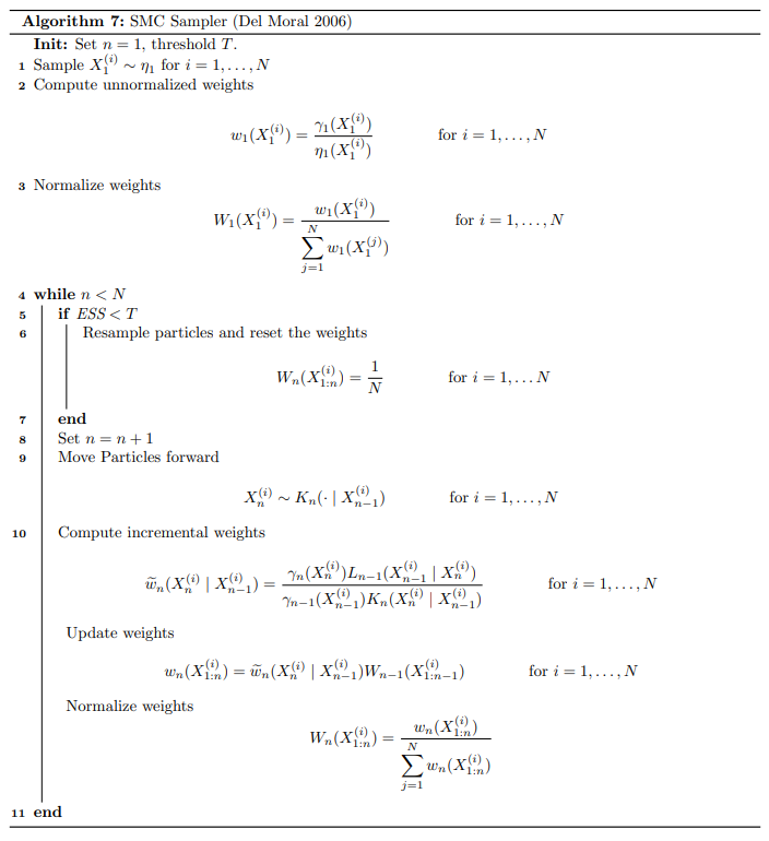
A few notes:
- The particle estimate of the $n$th target is $$ \pi_n^N(dx) = \sum_{i=1}^N W_n(X_{1:n}^{(i)}) \delta_{X_n^{(i)}}(dx) $$
- It is helpful to remember the distributions of $X_n^{(i)}$ and $X_{1:n}^{(i)}$ (using sloppy notation) \begin{align} X_n^{(i)} &\sim \int_{E^{n-1}} \eta_1(x_1) \prod_{k=2}^n K_k(x_k \mid x_{k-1}) dx_{1:k-1} \newline X_{1:n}^{(i)} &\sim \eta_1(x_1) \prod_{k=2}^{n} K_k(x_k \mid x_{k-1}) \end{align}
- The optimal backward kernel takes us back to IS on $E$ $$ L_{n-1}^{\text{opt}}(x_{n-1} \mid x_n) = \frac{\eta_{n-1}(x_{n-1}) K_n(x_n \mid x_{n-1})}{\eta_n(x_n)} $$ It is difficult to use this kernel as it relies on $\eta_{n-1}$ and $\eta_n$ which are intractable (indeed it is the reason why we went from SIS to SMC samplers).
- Sub-optimal kernel: substitute $\pi_n$ for $\eta_n$. This is motivated by the fact that, if $\eta_n$ is a good proposal for $\pi_n$ then they should be sufficiently close. First, rewrite the optimal kernel $$ L_{n-1}^{\text{opt}}(x_{n-1} \mid x_n) = \frac{\eta_{n-1}(x_{n-1}) K_n(x_n \mid x_{n-1})}{\eta_n(x_n)} = \frac{\eta_{n-1}(x_{n-1}) K_n(x_n \mid x_{n-1})}{\displaystyle \int_E \eta_{n-1}(x_{n-1}) K_n(x_n \mid x_{n-1}) dx_{n-1}} $$ Now substitute $\pi_n$ and $\pi_{n-1}$ for $\eta_n$ and $\eta_{n-1}$ respectively. $$ L_{n-1}(x_{n-1} \mid x_n) = \frac{\pi_{n-1}(x_{n-1}) K_n(x_n \mid x_{n-1})}{\displaystyle \int_E \pi_{n-1}(x_{n-1}) K_n(x_n \mid x_{n-1}) dx_{n-1}} $$ The incremental weights become \begin{align} w_n(x_n \mid x_{n-1}) &= \frac{\gamma_n(x_n) L_{n-1}(x_{n-1} \mid x_n)}{\gamma_{n-1}(x_{n-1}) K_n(x_n \mid x_{n-1})} \newline &= \frac{\gamma_n(x_n) \pi_{n-1}(x_{n-1}) K_n(x_n \mid x_{n-1})}{\gamma_{n-1}(x_{n-1}) K_n(x_n \mid x_{n-1}) \displaystyle \int_E \pi_{n-1}(x_{n-1}) K_n(x_n \mid x_{n-1}) dx_{n-1}} \end{align}
IS Measure Theory
Suppose $\pi_1: \mathcal{E} \to [0, 1]$ is our target probability distribution and $\eta_1: \mathcal{E} \to [0,1]$ is our IS proposal probability distribution. Suppose that they admit density with respect to the Lebesgue measure $dx$ on $(E, \mathcal{E})$ $$ \frac{d \pi_1}{d x} = \frac{\widetilde{p}_{\pi_1}(x)}{\displaystyle \int_E \widetilde{p}_{\pi_1}(y) dy} = p_{\pi_1}(x) \qquad \qquad \frac{d \eta_1}{d x}(x) = \frac{\widetilde{p}_{\eta_1}(x)}{\displaystyle \int_E \widetilde{p}_{\eta_1}(y) dy} = p_{\eta_1}(x) $$ Suppose that $\pi_1 \ll \eta_1$ then the Radon-Nikodym derivative of $\pi_1$ with respect to $\eta_1$ exists $$ \frac{d \pi_1}{d \eta_1} = \frac{w_1(x)}{\displaystyle \int_E w_1(x) d \eta_1(x)} $$ We can the approximate the expectation as follows \begin{align} \Ebb_{\pi_1}[\phi] &= \int_E \phi(x) d\pi_1(x) \newline &= \int_E \phi(x) \frac{d \pi_1}{d \eta_1}(x) d \eta_1(x) \newline &= \int_E \phi(x) \frac{d \pi_1}{d \eta_1}(x) \frac{d \eta_1}{dx}(x) dx \newline &= \frac{\displaystyle \int_E \phi(x) w_1(x) p_{\eta_1}(x) dx}{\displaystyle \int_E w_1(x) d\eta_1(x)} \newline &= \frac{\displaystyle \int_E \phi(x) w_1(x) p_{\eta_1}(x) dx}{\displaystyle \int_E w_1(x) \frac{d\eta_1}{dx}(x) dx} \newline &= \frac{\displaystyle \int_E \phi(x) w_1(x) p_{\eta_1}(x) dx}{\displaystyle \int_E w_1(x) p_{\eta_1}(x) dx} \end{align}
Now suppose you have samples $\{X_1^{(1:N)}\}\sim \eta_1$ then we can construct the particle approximation $$ \eta_1^N(dx) = \frac{1}{N} \sum_{i=1}^N \delta_{X_1^{(i)}}(dx) $$ Substituting this into the expression for the expectation we get \begin{align} \Ebb_{\pi_1}[\phi] &= \frac{\Ebb_{\eta_1}[\phi w_1]}{\Ebb_{\eta_1}[w_1]} \newline &\approx \frac{\Ebb_{\eta_1^N}[\phi w_1]}{\Ebb_{\eta_1^N}[w_1]} \newline &= \frac{\displaystyle \frac{1}{N} \sum_{i=1}^N \int_E \phi(x) w_1(x) \delta_{X_1^{(i)}}(dx)}{\displaystyle \frac{1}{N}\sum_{i=1}^N \int_E w_1(x) \delta_{X_1^{(i)}}(dx)} \newline &= \frac{\displaystyle \sum_{i=1}^N \phi(X_1^{(i)}) w_1(X_1^{(i)})}{\displaystyle \sum_{i=1}^N w_1(X_1^{(i)})} \newline &= \sum_{i=1}^N \phi(X_1^{(i)}) W_1(X_1^{(i)}) \end{align} where $$ W_1(X_1^{(i)}) = \frac{w_1(X_1^{(i)})}{\displaystyle \sum_{j=1}^N w_1(X_1^{(j)})} $$
SIS Proposal
Now let $K_n:E\times\mathcal{E}\to[0,1]$ be a Markov Kernel. Then this kernels can operate on the left with measures. $$ \eta_n = \eta_{n-1} K_n \implies \eta_n(A) = \int_E K_n(x, A) d \eta_{n-1}(x) = \int_E d \eta_{n-1}(x) \int_A K_n(x, dy) $$ Denote by $K_{n, x}:\mathcal{E} \to [0, 1]$ the probability measure in the second argument of the kernel, i.e. $K_{n, x}(A) = K_n(x, A)$ Suppose that $K_{n,x}$ admits a density with respect to the Lebesgue measure $$ \frac{d K_{n, x}}{dy}(y) = k_n(y \mid x) $$ Then the new measure can be written as \begin{align} \eta_n &= \int_E \frac{d \eta_{n-1}}{dx} \left[\int_A K_n(x, dy)\right] dx && \eta_{n-1} \ll dx\newline &= \int_E \frac{d \eta_{n-1}}{dx} \left[\int_A dK_{n, x}(y)\right] dx && \text{def } K_{n, x} \newline &= \int_E p_{\eta_{n-1}}(x) \left[\int_A \frac{d K_{n, x}(y)}{dy} dy\right] dx && K_{n, x} \ll dy\newline &= \int_E p_{\eta_{n-1}}(x) \left[\int_A k_n(y \mid x) dy\right] dx \newline &= \int_{E} \int_A p_{\eta_{n-1}}(x) k_n(y \mid x) dy dx \newline &= \int_{A} \left[\int_E p_{\eta_{n-1}}(x) k_n(y \mid x) dx \right] dy \end{align} Then by definition we must have that the expression in parenthesis is indeed the density of $\eta_n$ with respect to $dy$ $$ \frac{d \eta_n}{dy} = \int_E p_{\eta_{n-1}}(x) k_n(y \mid x) dx $$ Or more precisely, identifying $x = x_{n-1}$ and $y=x_n$ we have $$ p_{\eta_n}(x_n) = \frac{d \eta_n}{d x_n}(x_n) = \int_E p_{\eta_{n-1}}(x_{n-1}) k_n(x_n \mid x_{n-1}) dx_{n-1} $$ Indeed we have $$ \eta_n(A) = \int_A d \eta_n(x_n) = \int_A \frac{d \eta_n}{d x_n} dx_n = \int_A p_{\eta_n}(x_n) dx_n $$
SMC Proposal
The proposal in the SMC sampler is not given by $$ \eta_n = \eta_{n-1} K_n. $$ Indeed in SMC we don’t simply propose $X_n^{(i)}$. We propose $X_n^{(i)}$ and then we append it to $X_{1:n-1}^{(i)}$ which was generated according to $\eta_{n-1}$ and so on.
SMC Steps
- Step $n=1$: Our target is $\pi_1$ and proposal $\eta_1$ is given. Sample $X_1^{(1:N)} \sim \eta_1$. Weights are RN-derivative $$ w_1 \propto \frac{d \pi_1}{d \eta_1} $$
- Step $n=2$: Move particles forward using kernel $K_2: E\times\mathcal{E}\to[0,1]$. We sample $X_2^{(i)} \sim K_2(\cdot \mid X_1^{(i)})$. Marginally, each new particle $X_n^{(i)}$ is distributed as $$ X_{2}^{(i)} \sim \eta_2 = \eta_1 K_2 $$ Which can be written as \begin{align} \eta_2(A) &= \int_E d \eta_2 \newline &= \int_E d(\eta_1 K_2) \newline &= \int_E K_2(x_1, A) d \eta_1(x_1) \newline &= \int_E \int_A K_2(x_1, dx_2) \eta_1(x_1) \newline &= \int_E \left[\int_A \frac{d K_2(x_1, \cdot)}{dx_2} dx_2\right] \frac{d\eta_1(x_1)}{d x_1} dx_1 \newline &= \int_E \left[\int_A k_2(x_2 \mid x_1) dx_2\right] p_{\eta_1}(x_1) dx_1 \newline &= \int_E \int_A k_2(x_2 \mid x_1) p_{\eta_1}(x_1) dx_2 dx_1 \newline &= \int_A \left[\int_E k_2(x_2 \mid x_1) p_{\eta_1}(x_1) dx_1\right] dx_2 \end{align} where we can see that the density of $\eta_2$ is $$ \frac{d \eta_2}{d x_2}(x_2) = \int_E k_2(x_2 \mid x_1) p_{\eta_1}(x_1) dx_1. $$ In SMC we then append $X_2^{(i)}$ to $X_1^{(i)}$ to get $X_{1:2}^{(i)}$ so our aim is now to find a measure for it.
Define $\eta_{1:2}:= \eta \times K(x_1, \cdot)$ to be the following product measure on $\mathcal{E} \otimes \mathcal{E}$ $$ \eta_{1:2}(A\times B) := (\eta_1 \times K(x_1, \cdot))(A \times B) = \eta_1(A) K(x_1, B) \qquad A\times B \in \mathcal{E}\otimes \mathcal{E} \qquad x_1\in E $$ Since $\eta_1 \ll dx_1$ and $K(x_1, \cdot)\ll dx_2$ by a standard result (see here and here) on product measures we have that $\eta_{1:2} \ll d(x_1 \times x_2)$ and \begin{align} \frac{d \eta_{1:2}}{d(x_1 \times x_2)}(x_{1:2}) &= \frac{d (\eta_1 \times K(x_1, \cdot))}{d(x_1\times x_2)}(x_{1:2}) \newline &= \frac{d \eta_1}{d x_1}(x_1) \cdot \frac{d K(x_1, \cdot)}{dx_2}(x_2) \newline &= p_{\eta_1}(x_1) k_2(x_2 \mid x_1) \end{align} If we also define the extended target as the following product measure $$ \pi_{1:2}(A\times B) = (L_1(x_2, \cdot) \times \pi_2)(A, B) = L_1(x_2, A) \pi_2(B) $$ then by the same arguments as above its Radon-Nikodym derivative will be given by \begin{align} \frac{d \pi_{1:2}}{d (x_1 \times x_2)}(x_{1:2}) \newline &= \frac{d (L_1(x_2, \cdot) \times \pi_2)}{d (x_1 \times x_2)}(x_{1:2}) \newline &= \frac{d L_1(x_2, \cdot)}{d x_1}(x_1) \cdot \frac{d \pi_2}{d x_2}(x_2) \newline &= \ell(x_1 \mid x_2) p_{\pi_2}(x_2) \end{align} where $\ell$ is the density of $L$ with respect to $x_1$. As long as $\pi_{1:2} \ll \eta_{1:2}$ the weights are given by \begin{align} w_{1:2}(x_{1:2}) &= \frac{d \pi_{1:2}}{d \eta_{1:2}}(x_{1:2}) \newline &= \frac{d \pi_{1:2}}{d (x_1 \times x_2)} \cdot \frac{d (x_1 \times x_2)}{d \eta_{1:2}}(x_{1:2}) && \text{chain rule}\newline &= \frac{d \pi_{1:2}}{d (x_1 \times x_2)} \cdot \left(\frac{d \eta_{1:2}}{d (x_1 \times x_2)}\right)^{-1}(x_{1:2}) && \text{see below} \newline &= \frac{p_{\pi_2}(x_2) \ell(x_1 \mid x_2)}{p_{\eta_1}(x_1) k_2(x_2 \mid x_1)} \newline &= \frac{p_{\pi_2}(x_2) \ell(x_1 \mid x_2)}{p_{\pi_1}(x_1) k_2(x_2 \mid x_1)} \cdot \frac{p_{\pi_1}(x_1)}{p_{\eta_1}(x_1)} \newline &\propto \frac{\widetilde{p}_{\pi_2}(x_2) \ell(x_1 \mid x_2)}{\widetilde{p}_{\pi_1}(x_1) k_2(x_2 \mid x_1)} \cdot \frac{\widetilde{p}_{\pi_1}(x_1)}{\widetilde{p}_{\eta_1}(x_1)} \end{align} where on line $3$ we have used the following fact and on line $5$ we have basically multiplied by $1 = \frac{d \pi_1}{d\pi_1} = \frac{d \pi_1}{dx_1} \cdot \left(\frac{d \pi_1}{d x_1}\right)^{-1}$
- Step $n$: Target is $\pi_{1:n}$. Perform importance sampling using $\eta_{1:n}$ which is a product measure $$ \eta_{1:n} = \eta_1 \times K_n(x_{n-1}, \cdot) \times \cdots \times K_2(x_1, \cdot) $$ with density given by the product rule $$ \frac{d \eta_{1:n}}{d x_{1:n}} = p_{\eta_1}(x_1) \prod_{k=2}^n k_k(x_k \mid x_{k-1}) $$ Similarly the extended target is a product measure $$ \pi_{1:n} = \pi_n \times L_{n-1}(x_n, \cdot) \times \cdots \times L_1(x_1, \cdot) $$ with density $$ \frac{d \pi_{1:n}}{d x_{1:n}} = p_{\pi_n}(x_n) \prod_{k=1}^{n-1} \ell_k(x_k \mid x_{k+1}) $$ The weights are then given by $$ w_{1:n} = \frac{d \pi_{1:n}}{d \eta_{1:n}} \propto \frac{\widetilde{p}_{\pi_n}(x_n) \ell(x_{n-1} \mid x_n)}{\widetilde{p}_{\pi_{n-1}}(x_{n-1}) k_n(x_n \mid x_{n-1})} \cdot w_{1:n-1} $$