An introduction to Rejection ABC

$\newcommand{\ystar}{y^{*}} \newcommand{\Ycal}{\mathcal{Y}} \newcommand{\isample}{^{(i)}} \newcommand{\kernel}{p_{\epsilon}(\ystar \mid y)} \newcommand{\tkernel}{\tilde{p}_{\epsilon}(\ystar \mid y)} \newcommand{\jointABCpost}{p_{\epsilon}(\theta, y \mid \ystar)} \newcommand{\like}{p(y \mid \theta)} \newcommand{\prior}{p(\theta)} \newcommand{\truepost}{p(\theta \mid \ystar)} \newcommand{\ABCpost}{p_{\epsilon}(\theta \mid \ystar)} \newcommand{\ABClike}{p_{\epsilon}(\ystar \mid \theta)} \newcommand{\kerneltilde}{\tilde{p}_{\epsilon}(\ystar \mid y)} \newcommand{\zkernel}{Z_{\epsilon}} \newcommand{\truelike}{p(\ystar \mid \theta)}$

The Uniform Kernel: Rejection ABC

If we choose the ABC kernel to be a uniform kernel then we obtain Rejection-ABC. A uniform kernel is essentially an indicator function determining whether the true observation $\ystar$ is within an $\epsilon$-ball of the pseudo-observation $y\sim \like$ or not. $$ \kernel= \frac{1}{\text{Vol}(\epsilon)}\mathbb{I}_{B_{\epsilon}(y)}(\ystar) \propto \begin{cases} 1 & \ystar\in B_{\epsilon}(y) \ \newline 0 & \ystar \notin B_{\epsilon}(y) \end{cases} $$

In the expression above $B_{\epsilon}(y)$ is a ball of radius $\epsilon$ centered around the auxiliary data $y$: it contains all the data $y’\in \Ycal$ such that it is at a distance less than or equal to $\epsilon$, our tolerance. The distance is computed using a distance metric $\rho(\cdot, \cdot)$ which is usually the Euclidean one $$ B_{\epsilon}(y) = \left\{y’\in\Ycal \,\,: \,\, \rho(y, y’) \,\leq \, \epsilon\right\}. $$ The indicator function $\mathbb{I}_{B_{\epsilon}(y)}(\cdot)$ then is equal to $1$ whenever $\ystar$ is within an $\epsilon$-ball of $y$ and $0$ otherwise. Notice how we divide the indicator function by the $\text{Vol}(\epsilon)$, i.e. the volume of $B_{\epsilon}(y)$ so that the kernel is normalized and is thus a valid probability density function.

To sample $N$ parameters from $\truepost$ then we can follow the Rejection-ABC algorithm.

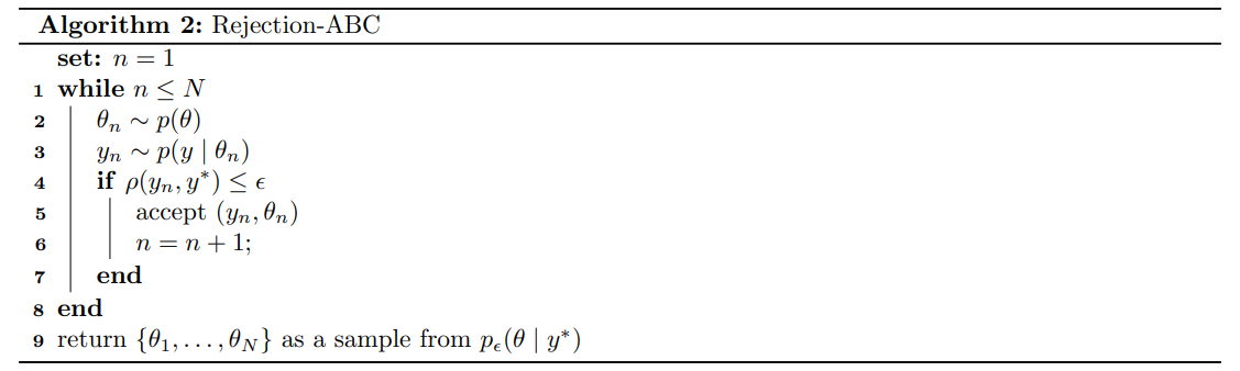
Essentially the choice of an indicator function as our kernel implicitly defines an algorithm that either rejects or accepts samples. To see this, notice that this is one of those cases where in practice we can only evaluate an unnormalized kernel $$ \tkernel = \mathbb{I}_{B_{\epsilon}(y)}(\ystar) $$ so that each $\tilde{w}_n$ is either $1$ or $0$. Suppose out of $w_1, \ldots, w_N$ there are only $M \leq N$ non-zero weights. Then their sum is clearly $M$ and so this algorithm can be interpreted similarly to Algorithm $1$ where $w_n = \frac{1}{M}$ when $\rho(y_n, \ystar) \leq \epsilon$.

Of course, this is extremely inefficient in high dimensions as the probability of “hitting the data” $\ystar$ with our $\epsilon$-ball $B_{\epsilon}(y)$ becomes negligible. If you compare this with Algorithm 1 you can see that accepted samples are those with weight of one $w_n=1$ while rejected samples have zero weight $w_n=0$.

As a side note, the posterior distribution targeted by Rejection Sampling is sometimes denoted $p(\theta \mid \rho(y, \ystar) \leq \epsilon)$ rather than the more general $\ABCpost$.

Two Moon Example

Again, we come back to the Two Moon example. Here is an example of how we could code a rejection sampler. Notice how I have set a maximum number of iterations to avoid the loop running indefinitely.

def rejection_abc(prior, simulator, distance, epsilon, N, y_star, maxiter=50):
    """General Rejection ABC Algorithm."""
    samples = np.zeros((N, len(y_star)))  # Accepted samples
    
    n = 0   # Number of accepted samples so far
    i = 0   # Number of iterations so far

    while (n < N) and (i < maxiter):

      # Sample from the prior
      theta_n = prior()

      # Run the simulator with new parameter
      y_n = simulator(theta_n)

      # Accept only if data is within epsilon distance from ystar
      if distance(y_n, y_star) <= epsilon:
          samples[n] = theta_n
          n += 1
          
      # Increase iteration count
      i += 1
    return samples

We can see below how Rejection ABC, imposing a “hard constraint”, gets fewer and fewer samples accepted as our tolerance $\epsilon$ becomes smaller.

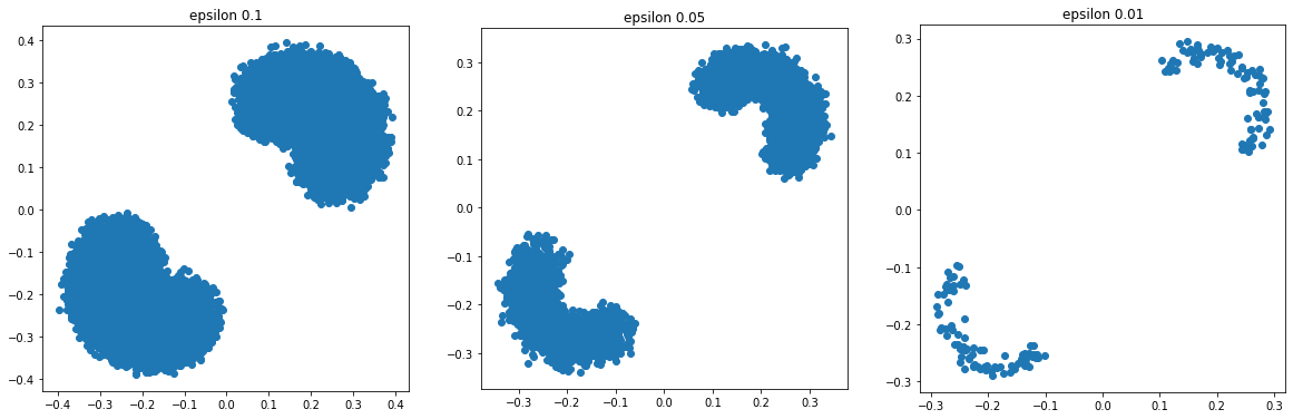
Once again, feel free to play around with this example with the following notebook.