Soft ABC

$\newcommand{\ystar}{y^{*}} \newcommand{\Ycal}{\mathcal{Y}} \newcommand{\isample}{^{(i)}} \newcommand{\kernel}{p_{\epsilon}(\ystar \mid y)} \newcommand{\tkernel}{\tilde{p}_{\epsilon}(\ystar \mid y)} \newcommand{\jointABCpost}{p_{\epsilon}(\theta, y \mid \ystar)} \newcommand{\like}{p(y \mid \theta)} \newcommand{\prior}{p(\theta)} \newcommand{\truepost}{p(\theta \mid \ystar)} \newcommand{\ABCpost}{p_{\epsilon}(\theta \mid \ystar)} \newcommand{\ABClike}{p_{\epsilon}(\ystar \mid \theta)} \newcommand{\kerneltilde}{\tilde{p}_{\epsilon}(\ystar \mid y)} \newcommand{\zkernel}{Z_{\epsilon}} \newcommand{\truelike}{p(\ystar \mid \theta)} \newcommand{\Ebb}{\mathbb{E}}$

A first ABC algorithm

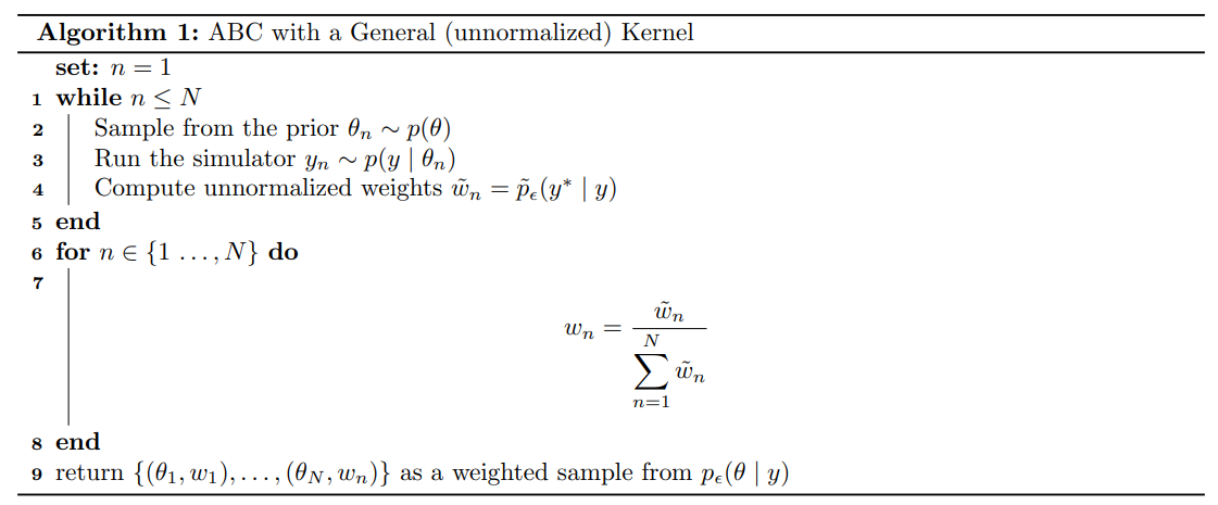
The algorithm that I hinted at in the earlier sections can be summarized as follows: At each iteration we first sample from the prior, we then run the simulator with the new parameter value and finally feed the output of the simulator in the kernel which will give us a weight representing the similarity between $y$ and $\ystar$. Sometimes we can only evaluate the kernel up to a normalizing constant, that is we can only compute $$ \tkernel \propto \kernel $$ In that case each weight will be un-normalized and so we will first compute all the weights and finally divide them by the sum of the weights, in a manner that resembles Importance Sampling.

This algorithm defines a posterior approximation as a mixture of Dirac deltas $$ \ABCpost = \sum_{i=n}^N w_n \delta_{\theta_n}(\theta) $$ and it can then be used, for example, to approximate the expectation of a function of $\theta$ with respect to theparameter posterior $$ \Ebb_{\truepost}\left[g(\theta)\right] \approx \Ebb_{\ABCpost}\left[g(\theta)\right] = \int g(\theta)\sum_{n=1}^N w_n \delta_{\theta_n}(\theta) d\theta = \sum_{n=1}^N g(\theta_n)w_n $$

In the next section, we will see a special case of this framework: Rejection ABC, where we choose the indicator function as our kernel function so that samples are assigned either a weight of $1$ or a weight of $0$, i.e. they are either accepted or rejected. This explains the name of the algorithm described above. We call Soft ABC in contrast to Rejection ABC which works with “hard rejections”, whereas Algorithm $1$ doesn’t reject, it simply assigns a weight.

Two Moon Example

The following example is taken from ‘APT for Likelihood-free Inference’. We consider the Two Moons simulator which, given $\theta\in\mathbb{R}^2$, produces data $y\in\mathbb{R}^2$ as follows $$ \begin{align} a &\sim \mathcal{U}\left(-\frac{\pi}{2}, \frac{\pi}{2}\right) \newline r &\sim \mathcal{N}(0.1, 0.01^2) \newline p &= (r\cos(a) + 0.25, r\sin(a))^\top \newline y &= p + \left(-\frac{|\theta_1 + \theta_2|}{\sqrt{2}}, \frac{-\theta_1 + \theta_2}{\sqrt{2}}\right) \end{align} $$ We also suppose that we have observed some data $\ystar = (0,0)^\top$. Notice how $a$ and $r$ are random variables that are generated inside the simulator and used for the sole purpose of generating data $y$ from $\theta$. These are called latent variables and they account for the stocasticity inside the simulator. We will talk more about these in a future lesson.

One could code the simulator in Python using the function below

def TM_simulator(theta):
    """Two Moons simulator for ABC."""
    t0, t1 = theta[0], theta[1]
    a = uniform(low=-np.pi/2, high=np.pi/2)
    r = normal(loc=0.1, scale=0.01)
    p = np.array([r * np.cos(a) + 0.25, r * np.sin(a)])
    return p + np.array([-np.abs(t0 + t1), (-t0 + t1)]) / sqrt(2)

and the Soft-ABC algorithm could like as follows:

def soft_abc(prior, simulator, kernel, epsilon, N, y_star):
    """Soft ABC algorithm."""
    samples = np.zeros((N, len(y_star)))       # Store samples
    weights = np.zeros(N)                      # Store weights  

    n = 0                                      # Number of iterations

    while n < N:

      theta_n = prior()                        # Sample from the prior
      y_n = simulator(theta_n)                 # Run the simulator
      w_n_tilde = kernel(y_n, y_star, epsilon) # Unnormalized weights

      # Store samples and unnormalized weights
      samples[n] = theta_n
      weights[n] = w_n_tilde

      n += 1

    # Normalize weights
    weights = weights / np.sum(weights)

    # Return weighted samples
    return samples, weights

Using $0.1, 0.05, 0.01$ as epsilon values these are the results I obtained.

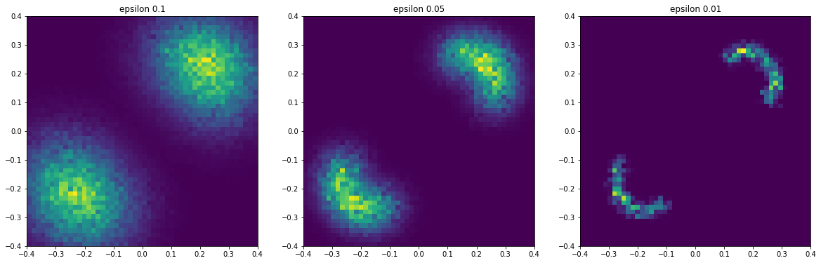
Above I have plotted the samples as histograms where the weights are given by the normalized soft-abc weights. We can see that as epsilon gets smaller, we are getting more accurate and placing more importance on data that is closer to the observed data $\ystar=(0, 0)^\top$.

If you would like to play around with this example, you can find a tutorial Google Colab notebook here.