Comparing Original Images with their Reconstructions

Now it’s time to see what our reconstructions look like. Notice from the code block above that the last testing batch of images and their reconstructions are saved in the test_images and reconstructions variables. These have shape [100, 1, 28, 28] and [100, 784] respectively. What follows may look a bit messy but we are essentially doing the following operations for both sets of images:

• Send tensor to CPU via .cpu(). This is needed because we cannot transform a tensor to numpy when the tensor is saved on GPU. Therefore we first move it to CPU and then transform it to numpy.
• We “clamp” or “clip” the values to be between 0 and 1. This means that values above 1 are set to 1. Values below 0 are set to 0 and values in between are kept the same. This shouldn’t be necessary due to the sigmoid function, but we still do it for good practice.
• We select only the first 50 images.
• We generate a grid of 5 images by 10 images.
• Finally we transform the tensor to Numpy and shape it correctly to be displayed by plt.imshow().

# Display original images
with torch.no_grad():
    print("Original Images")
    test_images = test_images.cpu()
    test_images = test_images.clamp(0, 1)
    test_images = test_images[:50]
    test_images = make_grid(test_images, 10, 5)
    test_images = test_images.numpy()
    test_images = np.transpose(test_images, (1, 2, 0))
    plt.imshow(test_images)
    plt.show()

# Display reconstructed images
with torch.no_grad():
    print("Reconstructions")
    reconstructions = reconstructions.view(reconstructions.size(0), 1, 28, 28)
    reconstructions = reconstructions.cpu()
    reconstructions = reconstructions.clamp(0, 1)
    reconstructions = reconstructions[:50]
    plt.imshow(np.transpose(make_grid(reconstructions, 10, 5).numpy(), (1, 2, 0)))
    plt.show()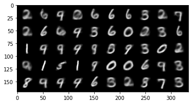

Pytorch VAE Testing

We can now assess its performance on the test set. There are a few key points to notice, which are discussed also here:

• vae.eval() will tell every layer of the VAE that we are in evaluation mode. In general, this means that dropout and batch normalization layers will work in evaluation mode. In this particular example, vae.eval() will make sure that we are not sampling from the latent space, but we are simply using mu.
• torch.no_grad() tells VAE that it doesn’t need to keep track of gradients, which speeds up evaluation.

# Set VAE to evaluation mode (deactivates potential dropout layers)
# So that we use the latent mean and we don't sample from the latent space
vae.eval()

# Keep track of test loss (notice, we have no epochs)
test_loss, number_of_batches = 0.0, 0

for test_images, _ in testloader:

  # Do not track gradients
  with torch.no_grad():

    # Send images to the GPU/CPU
    test_images = test_images.to(device)

    # Feed images through the VAE to obtain their reconstruction & compute loss
    reconstructions, latent_mu, latent_logvar = vae(test_images)
    loss = vae_loss(test_images, reconstructions, latent_mu, latent_logvar)

    # Cumulative loss & Number of batches
    test_loss += loss.item()
    number_of_batches += 1

# Now divide by number of batches to get average loss per batch
test_loss /= number_of_batches
print('average reconstruction error: %f' % (test_loss))

Depending on how many epochs we trained for, we should find a similar loss as to the training set, showing that the network has learned.

average reconstruction error: 15142.687080

Separating Encoder and Decoder in VAE

With our minimalist version of the Variational Autoencoder, we cannot sample an image or visualize what the latent space looks like. To sample an image we would need to sample from the latent space and then feed this into the “decoder” part of the VAE. To visualize what the latent space looks like we would need to create a grid in the latent space and then feed each latent vector into the decoder to see what the images at each grid point look like. Unfortunately we cannot easily split our network as it currently is. This is why most implementations of the VAE that you will likely find online will separate the encoder and the decoder either as two different methods of the VAE or even as two different classes, each inheriting from nn.Module. For instance, this version of the VAE would allow you to sample images and visualize the latent space:

class VAE(nn.Module):
    def __init__(self):
        """Variational Auto-Encoder Class"""
        super(VAE, self).__init__()
        # Encoding Layers
        self.e_input2hidden = nn.Linear(in_features=784, out_features=e_hidden)
        self.e_hidden2mean = nn.Linear(in_features=e_hidden, out_features=latent_dim)
        self.e_hidden2logvar = nn.Linear(in_features=e_hidden, out_features=latent_dim)
        
        # Decoding Layers
        self.d_latent2hidden = nn.Linear(in_features=latent_dim, out_features=d_hidden)
        self.d_hidden2image = nn.Linear(in_features=d_hidden, out_features=784)
        
    def encoder(self, x):
        # Shape Flatten image to [batch_size, input_features]
        x = x.view(-1, 784)
        # Feed x into Encoder to obtain mean and logvar
        x = F.relu(self.e_input2hidden(x))
        return self.e_hidden2mean(x), self.e_hidden2logvar(x)
        
    def decoder(self, z):
        return torch.sigmoid(self.d_hidden2image(torch.relu(self.d_latent2hidden(z))))
        
    def forward(self, x):
        # Encoder image to latent representation mean & std
        mu, logvar = self.encoder(x)
        
        # Sample z from latent space using mu and logvar
        if self.training:
            z = torch.randn_like(mu).mul(torch.exp(0.5*logvar)).add_(mu)
        else:
            z = mu
        
        # Feed z into Decoder to obtain reconstructed image. Use Sigmoid as output activation (=probabilities)
        x_recon = self.decoder(z)
        
        return x_recon, mu, logvar

Data Generation

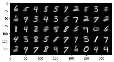
To sample images from the generative model we can do something like this. Notice how we set the VAE in evaluation mode and we make sure that Pytorch doesn’t keep track of gradients. All we do is sampling an array with shape [50, latent_dim] of standard normal variates, making sure that this tensor is saved to GPU. Then, we feed it through the decoder, obtaining a reconstruction, we reshape it the correct image shape. The rest, is just the usual trick to print images from Pytorch GPU with matplotlib.

vae.eval()
with torch.no_grad():
    # Sample from standard normal distribution
    z = torch.randn(50, latent_dim, device=device)
    
    # Reconstruct images from sampled latent vectors
    recon_images = vae.decoder(z)
    recon_images = recon_images.view(recon_images.size(0), 1, 28, 28)
    recon_images = recon_images.cpu()
    recon_images = recon_images.clamp(0, 1)
    
    # Plot Generated Images
    plt.imshow(np.transpose(make_grid(recon_images, 10, 5).numpy(), (1, 2, 0)))

The result should look something like this, depending on the number of epochs:

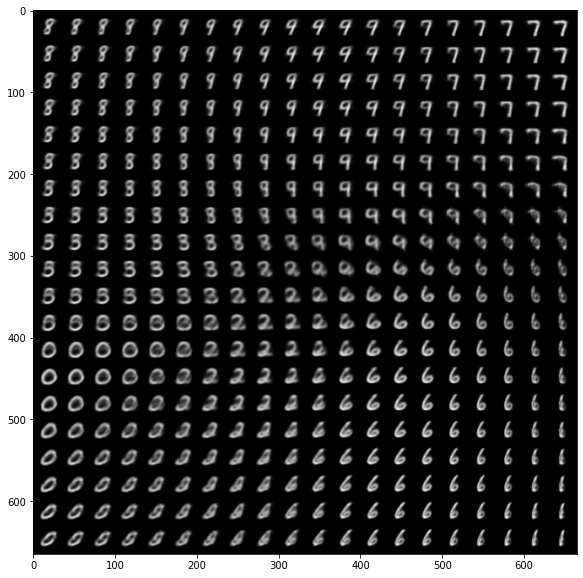
Finally, we can also visualize the latent space. Notice that since we are using simple linear layers and very few epochs, this will look very messy. For better performance we would need to use convolutional layers in the encoder & decoder.

with torch.no_grad():
  # Create empty (x, y) grid
  latent_x = np.linspace(-1.5, 1.5, 20)
  latent_y = np.linspace(-1.5, 1.5, 20)
  latents = torch.FloatTensor(len(latent_x), len(latent_y), 2)
  # Fill up the grid
  for i, lx in enumerate(latent_x):
    for j, ly in enumerate(latent_y):
      latents[j, i, 0] = lx
      latents[j, i, 1] = ly
  # Flatten the grid
  latents = latents.view(-1, 2)
  # Send to GPU
  latents = latents.to(device)
  # Find their representation
  reconstructions = vae.decoder(latents).view(-1, 1, 28, 28)
  reconstructions = reconstructions.cpu()
  # Finally, plot
  fig, ax = plt.subplots(figsize=(10, 10))
  plt.imshow(np.transpose(make_grid(reconstructions.data[:400], 20, 5).clamp(0, 1).numpy(), (1, 2, 0))) 

Basically we are generating a grid of values in the latent space. Then we are decoding the grid into images, reshaping it and plotting it. The result, looks like this:

In order to write the code here I made use of a few resources. Firstly, Kingma is a great example of a minimalist variational autoencoder. In addition, this implementation by Federico Bergamin was extremely helpful in clarifying what does what. Last but not least, this Google Colab notebook helped me work out how to display the latent space and how to generate images from the VAE.

You can find the code used here in this Google Colab notebook.

Bibliography

Durk Kingma. 2020. “Variational Autoencoder in Pytorch.” https://github.com/dpkingma/examples/blob/master/vae/main.py.
Federico Bergamin. 2020. “Variational-Autoencoders.” https://github.com/federicobergamin/Variational-Autoencoders/blob/master/VAE.py.
Paul Guerrero, Nils Thuerey. 2020. “Smart Geometry Ucl - Variational Autoencoder Pytorch.” https://colab.research.google.com/github/smartgeometry-ucl/dl4g/blob/master/variational_autoencoder.ipynb#scrollTo=TglLFCT1N7iF.
Mauro Camara Escudero
Machine Learning Engineer
My research interests include approximate manifold sampling and generative models.