Latent Variable Models (LVM)

Suppose we observe some data \(\mathcal{D}= \{\boldsymbol{\mathbf{x}}_1, \ldots, \boldsymbol{\mathbf{x}}_N\}\). Often we know that what we have observed is only part of the whole picture, and to understand the system at hand we have to introduce some latent variables. Consider, for now, a single data point \(\boldsymbol{\mathbf{x}}\) and its corresponding latent variables \(\boldsymbol{\mathbf{z}}\). Then, we might be interested in the following three tasks.

• Generative Modelling: Generating samples from the following distributions, efficiently. \[ p_{\boldsymbol{\mathbf{\theta}}}(\boldsymbol{\mathbf{x}})= \int p_{\boldsymbol{\mathbf{\theta}}}(\boldsymbol{\mathbf{x}}, \boldsymbol{\mathbf{z}})d\boldsymbol{\mathbf{z}} \]
• Posterior Inference: Modelling the posterior distribution over the latent variables. \[ p_{\boldsymbol{\mathbf{\theta}}}(\boldsymbol{\mathbf{z}}\mid \boldsymbol{\mathbf{x}})= \frac{p_{\boldsymbol{\mathbf{\theta}}}(\boldsymbol{\mathbf{x}}, \boldsymbol{\mathbf{z}})}{p_{\boldsymbol{\mathbf{\theta}}}(\boldsymbol{\mathbf{x}})} \]
• Parameter Estimation: Performing Maximum Likelihood Estimation (MLE) or Maximum-A-Posteriori estimation (MAP) for the parameter \(\boldsymbol{\mathbf{\theta}}\): \[ \boldsymbol{\mathbf{\theta}}^{*}= \arg \max_{\boldsymbol{\mathbf{\theta}}} \prod_{\boldsymbol{\mathbf{x}}\in\mathcal{D}}p_{\boldsymbol{\mathbf{\theta}}}(\boldsymbol{\mathbf{x}})\quad \text{or} \quad \boldsymbol{\mathbf{\theta}}^{*} = \arg\max_{\boldsymbol{\mathbf{\theta}}} \left[\prod_{\boldsymbol{\mathbf{x}}\in\mathcal{D}}p_{\boldsymbol{\mathbf{\theta}}}(\boldsymbol{\mathbf{x}})\right]p(\boldsymbol{\mathbf{\theta}}) \]

The settings and problems described above are quite standard and of widespread interest. One method to perform Maximum Likelihood Estimation in Latent Variable Models is the Expectation-Maximization algorithm, while a method to perform posterior inference is Mean-Field Variational Inference.

Expectation-Maximization Algorithm for Maximum Likelihood Estimation

Suppose that, for some reason, we have a fairly good estimate for the parameter, let’s call this guess \(\widehat{\boldsymbol{\mathbf{\theta}}}\). How can we improve this guess? One way to go about this is to use \(\widehat{\boldsymbol{\mathbf{\theta}}}\) to construct the posterior distribution at each data point \[ \left\{p_{\widehat{\boldsymbol{\mathbf{\theta}}}}(\boldsymbol{\mathbf{z}}\mid \boldsymbol{\mathbf{x}}) \,\,:\,\, \boldsymbol{\mathbf{x}}\in\mathcal{D}\right\} \] And then we find an updated and improved parameter value by maximizing the expected complete-data log likelihood \[ \arg\max_{\boldsymbol{\mathbf{\theta}}} \mathbb{E}_{p_{\widehat{\boldsymbol{\mathbf{\theta}}}}(\boldsymbol{\mathbf{z}}\mid \boldsymbol{\mathbf{x}})}\left[\log p_{\boldsymbol{\mathbf{\theta}}}(\boldsymbol{\mathbf{x}}, \boldsymbol{\mathbf{z}})\right] \] That is, rather than maximizing the incomplete-data likelihood \(p_{\widehat{\boldsymbol{\mathbf{\theta}}}}(\boldsymbol{\mathbf{x}})\), we maximize the joint likelihood \(p_{\widehat{\boldsymbol{\mathbf{\theta}}}}(\boldsymbol{\mathbf{x}}, \boldsymbol{\mathbf{z}})\), but since we don’t actually have the latent variables \(\boldsymbol{\mathbf{z}}\) we average this complete-data likelihood with respect to the posterior of the latent variables given the data and the parameter value \(p_{\widehat{\boldsymbol{\mathbf{\theta}}}}(\boldsymbol{\mathbf{z}}\mid\boldsymbol{\mathbf{x}})\). By iterating this proceedure we obtain the following algorithm.

• Initialize \(\boldsymbol{\mathbf{\theta}}^{(0)}\) and set \(t=0\).
• Until convergence:
  • Compute posterior distribution of the latent variables given the observations \[ \left\{p_{\boldsymbol{\mathbf{\theta}}^{(t)}}(\boldsymbol{\mathbf{z}}\mid \boldsymbol{\mathbf{x}}) \,\,:\,\, \boldsymbol{\mathbf{x}}\in\mathcal{D}\right\} \]
  • Choose new parameter value \(\boldsymbol{\mathbf{\theta}}^{(t+1)}\) so that it maximises \[ \sum_{\boldsymbol{\mathbf{x}}\in\mathcal{D}} \mathbb{E}_{p_{\boldsymbol{\mathbf{\theta}}^{(t)}}(\boldsymbol{\mathbf{z}}\mid \boldsymbol{\mathbf{x}})}\left[\log p_{\boldsymbol{\mathbf{\theta}}}(\boldsymbol{\mathbf{x}}, \boldsymbol{\mathbf{z}})\right] \]

Problem: The EM Algorithm breaks if \(p_{\boldsymbol{\mathbf{\theta}}^{(t)}}(\boldsymbol{\mathbf{z}}\mid \boldsymbol{\mathbf{x}})\) are intractable.

Mean-Field Variational Inference for Posterior Inference

A well-known method, alternative to MCMC, for posterior inference if Mean-Field Variational Inference. In Variational Inference we essentially define a family of distributions that we think is somehow representative of the true posterior distribution \(p_{\boldsymbol{\mathbf{\theta}}}(\boldsymbol{\mathbf{z}}\mid \boldsymbol{\mathbf{x}})\). Then, we choose the member of that family that is closest, in some sense, to the true posterior. In Mean-Field Variational Inference we assume that such a family of distributions is factorized into a product of terms, one for each data point.

\[ \prod_{i=1}^{N} q_{\boldsymbol{\mathbf{\phi}}_i}(\boldsymbol{\mathbf{z}}_i) \approx \prod_{i=1}^N p_{\boldsymbol{\mathbf{\theta}}}(\boldsymbol{\mathbf{z}}_i \mid \boldsymbol{\mathbf{x}}) \]

We can see that each factor in the product on the RHS is described by a vector of parameters \(\boldsymbol{\mathbf{\phi}}_i\). Usually, to judge how close each member of the chosen family is to the true posterior, we use the KL-divergence. This means that we need to solve an optimization problem for each factor in the approximation, i.e. for each data point \[ \boldsymbol{\mathbf{\phi}}^*_i = \arg\min_{\boldsymbol{\mathbf{\phi}}_i} \text{KL}(q_{\boldsymbol{\mathbf{\phi}}_i}(\boldsymbol{\mathbf{z}}\mid\boldsymbol{\mathbf{x}})\,\,||\,\,p_{\boldsymbol{\mathbf{\theta}}}(\boldsymbol{\mathbf{z}}\mid \boldsymbol{\mathbf{x}})). \]

Problem: It clearly doesn’t scale well with large datasets and it breaks if \(\mathbb{E}_{q_{\boldsymbol{\mathbf{\phi}}_i}}\left[\cdot\right]\) are intractable.

Ideally, we would like to use only one vector of parameter \(\boldsymbol{\mathbf{\phi}}\), which is shared across data points. This is called amortized inference.

Variational Autoencoders at a Glance

So what are Variational Autoencoders or Auto-Encoding Variational Bayes?? Below is a summary of what they are and what they are used for.

• What is AEVB used for? Inference and Generative Modelling in LVMs.
• How do AEVBs work? Optimization of an unbiased estimator of an objective function using SGD.
• What are VAEs? They are AEVB where the probability distributions in the LVM are parametrized by Neural Networks.

Auto-Encoding Variational Bayes Objective Function

In this section, we derive the objective function of AEVB. First, let us introduce a so-called recognition model \(q_{\boldsymbol{\mathbf{\phi}}}(\boldsymbol{\mathbf{z}}\mid\boldsymbol{\mathbf{x}})\). This is a chosen distribution that we want to use to approximate the true posterior distribution \(p_{\boldsymbol{\mathbf{\theta}}}(\boldsymbol{\mathbf{z}}\mid \boldsymbol{\mathbf{x}})\), similar to how we did it for Mean-Field Variational Inference. The key difference here is that instead of having a different vector of parameters for each data point, we share a single vector of parameters across data points. Then, we consider the KL divergence between this approximating distribution and the true posterior

\[\begin{align*} \text{KL}(q_{\boldsymbol{\mathbf{\phi}}}(\boldsymbol{\mathbf{z}}\mid \boldsymbol{\mathbf{x}})\,\,||\,\,p_{\boldsymbol{\mathbf{\theta}}}(\boldsymbol{\mathbf{z}}\mid \boldsymbol{\mathbf{x}})) &= \mathbb{E}_{q_{\boldsymbol{\mathbf{\phi}}}}\left[\log q_{\boldsymbol{\mathbf{\phi}}}(\boldsymbol{\mathbf{z}}\mid \boldsymbol{\mathbf{x}})- \log p_{\boldsymbol{\mathbf{\theta}}}(\boldsymbol{\mathbf{z}}\mid \boldsymbol{\mathbf{x}})\right] \\ &= -\mathbb{E}_{q_{\boldsymbol{\mathbf{\phi}}}}\left[\log\left(\frac{p_{\boldsymbol{\mathbf{\theta}}}(\boldsymbol{\mathbf{x}}, \boldsymbol{\mathbf{z}})}{q_{\boldsymbol{\mathbf{\phi}}}(\boldsymbol{\mathbf{z}}\mid \boldsymbol{\mathbf{x}})}\right)\right] + \log p_{\boldsymbol{\mathbf{\theta}}}(\boldsymbol{\mathbf{x}})\\ &:= -\mathcal{L}_{\theta, \boldsymbol{\mathbf{\phi}}}(\boldsymbol{\mathbf{x}})+ \log p_{\boldsymbol{\mathbf{\theta}}}(\boldsymbol{\mathbf{x}}) \end{align*}\]

Notice how we managed to write the KL divergence in terms of the log marginal likelihood \(p_{\boldsymbol{\mathbf{\theta}}}(\boldsymbol{\mathbf{x}})\) and a term that we call \(\mathcal{L}_{\theta, \boldsymbol{\mathbf{\phi}}}(\boldsymbol{\mathbf{x}})\). We can now rearrange the following expression and notice that, since the KL divergence is always non-negative, \(\mathcal{L}_{\theta, \boldsymbol{\mathbf{\phi}}}(\boldsymbol{\mathbf{x}})\) provides a lower bound for the marginal log-likelihood.

\[\begin{align*} \log p_{\boldsymbol{\mathbf{\theta}}}(\boldsymbol{\mathbf{x}}) &= \text{KL}(q_{\boldsymbol{\mathbf{\phi}}}(\boldsymbol{\mathbf{z}}\mid \boldsymbol{\mathbf{x}})\,\,||\,\,p_{\boldsymbol{\mathbf{\theta}}}(\boldsymbol{\mathbf{z}}\mid \boldsymbol{\mathbf{x}})) + \mathcal{L}_{\theta, \boldsymbol{\mathbf{\phi}}}(\boldsymbol{\mathbf{x}})\\ &\geq \mathcal{L}_{\theta, \boldsymbol{\mathbf{\phi}}}(\boldsymbol{\mathbf{x}}) \end{align*}\]

For this reason, we call \(\mathcal{L}_{\theta, \boldsymbol{\mathbf{\phi}}}(\boldsymbol{\mathbf{x}})\) the Evidence Lower BOund (ELBO). With an i.i.d dataset we can see that this relationships holds for the whole dataset:

\[ \sum_{\boldsymbol{\mathbf{x}}\in\mathcal{D}} \log p_{\boldsymbol{\mathbf{\theta}}}(\boldsymbol{\mathbf{x}})\geq \sum_{\boldsymbol{\mathbf{x}}\in\mathcal{D}} \mathcal{L}_{\theta, \boldsymbol{\mathbf{\phi}}}(\boldsymbol{\mathbf{x}}) \]

Why is it useful to find a lower bound on the log marginal likelihood? Because by maximizing the ELBO we get two birds with one stone. First of all, notice how by maximizing the ELBO with respect to \(\boldsymbol{\mathbf{\theta}}\), we can expect to approximately maximize also the log marginal likelihood. Similarly, by maximizing the ELBO with respect to \(\boldsymbol{\mathbf{\phi}}\) we can see that, since the ELBO can be written as the log marginal likelihood minus the kl divergence, this is equivalent to minimizing the KL divergence. In summary we can write:

\[\begin{equation*} \max_{\boldsymbol{\mathbf{\theta}}, \boldsymbol{\mathbf{\phi}}} \mathcal{L}_{\theta, \boldsymbol{\mathbf{\phi}}}(\boldsymbol{\mathbf{x}})\implies \begin{cases} \displaystyle\max_{\boldsymbol{\mathbf{\theta}}} \sum_{\boldsymbol{\mathbf{x}}\in\mathcal{D}}\log p_{\boldsymbol{\mathbf{\theta}}}(\boldsymbol{\mathbf{x}})& \text{as } \log p_{\boldsymbol{\mathbf{\theta}}}(\boldsymbol{\mathbf{x}})\geq \mathcal{L}_{\theta, \boldsymbol{\mathbf{\phi}}}(\boldsymbol{\mathbf{x}})\\ \displaystyle\min_{\boldsymbol{\mathbf{\phi}}} \sum_{\boldsymbol{\mathbf{x}}\in\mathcal{D}} \text{KL} & \text{as } \log p_{\boldsymbol{\mathbf{\theta}}}(\boldsymbol{\mathbf{x}})-\text{KL} = \mathcal{L}_{\theta, \boldsymbol{\mathbf{\phi}}}(\boldsymbol{\mathbf{x}}) \end{cases} \end{equation*}\]

Repectively, such maximization have a very practical results:

• The generative model \(p_{\boldsymbol{\mathbf{\theta}}}(\boldsymbol{\mathbf{x}})\) improves.
• The approximation \(q_{\boldsymbol{\mathbf{\phi}}}(\boldsymbol{\mathbf{z}}\mid \boldsymbol{\mathbf{x}})\) improves.

Lastly, one can also write the ELBO in a different way. This second formulation is often convenient because it will tend to have estimates with lower variance.

\[\begin{align*} \mathcal{L}_{\theta, \boldsymbol{\mathbf{\phi}}}(\boldsymbol{\mathbf{x}}) &= \log p_{\boldsymbol{\mathbf{\theta}}}(\boldsymbol{\mathbf{x}})- \text{KL}(q_{\boldsymbol{\mathbf{\phi}}}\,\,||\,\,p_{\boldsymbol{\mathbf{\theta}}}(\boldsymbol{\mathbf{z}}\mid \boldsymbol{\mathbf{x}})) \\ &= \mathbb{E}_{q_{\boldsymbol{\mathbf{\phi}}}}\left[ \log \left(p_{\boldsymbol{\mathbf{\theta}}}(\boldsymbol{\mathbf{x}}\mid \boldsymbol{\mathbf{z}})p_{\boldsymbol{\mathbf{\theta}}}(\boldsymbol{\mathbf{z}})\right)- \log q_{\boldsymbol{\mathbf{\phi}}}(\boldsymbol{\mathbf{z}}\mid \boldsymbol{\mathbf{x}})\right] \\ &= \underbrace{\mathbb{E}_{q_{\boldsymbol{\mathbf{\phi}}}}\left[\log p_{\boldsymbol{\mathbf{\theta}}}(\boldsymbol{\mathbf{x}}\mid \boldsymbol{\mathbf{z}})\right]}_{\text{Expected Reconstruction Error}} - \underbrace{\text{KL}(q_{\boldsymbol{\mathbf{\phi}}}(\boldsymbol{\mathbf{z}}\mid \boldsymbol{\mathbf{x}})\,\,||\,\,p_{\boldsymbol{\mathbf{\theta}}}(\boldsymbol{\mathbf{z}}))}_{\text{Regularization Term}} \end{align*}\]

As can be seen above, the ELBO can be written as a sum of two terms: expected reconstruction error and the KL divergence between the approximation and the latent prior. This KL-divergence can be interpreted as a regularization term trying to keep the approximation close to the prior. This regularization term can sometimes backfire and maintain the approximation to be exactly equal to the prior. To deal with such scenarios, called posterior collapse, people have been developing new methods, such as delta-VAEs.

Optimization of the ELBO Objective Function

One way to optimize the ELBO with respect to \(\boldsymbol{\mathbf{\phi}}\) and \(\boldsymbol{\mathbf{\theta}}\) is to perform gradient descent. Since our aim is to find an algorithm that scales well with large datasets, we want to use Stochastic Gradient Ascent. In order to do so, we need to be able to compute \(\nabla_{\boldsymbol{\mathbf{\phi}}} \mathcal{L}_{\theta, \boldsymbol{\mathbf{\phi}}}(\boldsymbol{\mathbf{x}})\) and \(\nabla_{\boldsymbol{\mathbf{\theta}}}\mathcal{L}_{\theta, \boldsymbol{\mathbf{\phi}}}(\boldsymbol{\mathbf{x}})\). However, notice how in both formulations of the ELBO we find expectations with respect to \(q_{\boldsymbol{\mathbf{\phi}}}(\boldsymbol{\mathbf{z}}\mid \boldsymbol{\mathbf{x}})\), which depends on \(\boldsymbol{\mathbf{\phi}}\)

\[\begin{equation*} \mathcal{L}_{\theta, \boldsymbol{\mathbf{\phi}}}(\boldsymbol{\mathbf{x}})= \begin{cases} \displaystyle \mathbb{E}_{q_{\boldsymbol{\mathbf{\phi}}}}\left[\log p_{\boldsymbol{\mathbf{\theta}}}(\boldsymbol{\mathbf{x}}, \boldsymbol{\mathbf{z}})- \log q_{\boldsymbol{\mathbf{\phi}}}(\boldsymbol{\mathbf{z}}\mid \boldsymbol{\mathbf{x}})\right] \\ \qquad \\ \displaystyle \mathbb{E}_{q_{\boldsymbol{\mathbf{\phi}}}}\left[\log p_{\boldsymbol{\mathbf{\theta}}}(\boldsymbol{\mathbf{x}}\mid \boldsymbol{\mathbf{z}})\right] - \text{KL}(q_{\boldsymbol{\mathbf{\phi}}}\,\,||\,\,p_{\boldsymbol{\mathbf{\theta}}}(\boldsymbol{\mathbf{z}})) \end{cases} \end{equation*}\]

This means that when taking the gradient of the ELBO with respect to \(\boldsymbol{\mathbf{\phi}}\) we cannot exchange the gradient and the expectation sign

\[ \nabla_{\boldsymbol{\mathbf{\phi}}}\mathbb{E}_{q_{\boldsymbol{\mathbf{\phi}}}(\boldsymbol{\mathbf{z}}\mid \boldsymbol{\mathbf{x}})}\left[ \cdot \right] \neq \mathbb{E}_{q_{\boldsymbol{\mathbf{\phi}}}(\boldsymbol{\mathbf{z}}\mid \boldsymbol{\mathbf{x}})}\left[\nabla_{\boldsymbol{\mathbf{\phi}}} \right] \] We would like to do this “exchange” operation so that we can approximate the gradient with a simple Monte Carlo estimate as it is usually done in Stochastic Gradient Ascent. To go around this problem our question becomes:

Can we write the expectation with respect to a distribution that is independent of \(\boldsymbol{\mathbf{\phi}}\)? \[ \nabla_{\boldsymbol{\mathbf{\phi}}}\mathbb{E}_{q_{\boldsymbol{\mathbf{\phi}}}(\boldsymbol{\mathbf{z}}\mid \boldsymbol{\mathbf{x}})}\left[\cdot\right] = \mathbb{E}_{p(\boldsymbol{\mathbf{\epsilon}})}\left[\nabla_{\boldsymbol{\mathbf{\phi}}}\right] \]

If we think about it, we already know a special case in which this can be done. For instance, suppose that the distribution \(q_{\boldsymbol{\mathbf{\phi}}}(\boldsymbol{\mathbf{z}}\mid \boldsymbol{\mathbf{x}})\) is actually a multivariate normal distribution \(\mathcal{N}(\boldsymbol{\mathbf{\mu}}, \boldsymbol{\mathbf{\Sigma}})\). Then, we can rewrite a sample \(\boldsymbol{\mathbf{z}}\sim q_{\boldsymbol{\mathbf{\phi}}}(\boldsymbol{\mathbf{z}}\mid \boldsymbol{\mathbf{x}})\) in terms of a standard multivariate normal distribution \[ \boldsymbol{\mathbf{z}}= \boldsymbol{\mathbf{\mu}}+ \boldsymbol{\mathbf{L}}\boldsymbol{\mathbf{\epsilon}}\qquad \text{where} \qquad \boldsymbol{\mathbf{\epsilon}}\sim \mathcal{N}(\boldsymbol{\mathbf{0}}, \boldsymbol{\mathbf{I}}) \] where \(\boldsymbol{\mathbf{L}}\boldsymbol{\mathbf{L}}^\top\) is the Cholesky decomposition of \(\boldsymbol{\mathbf{\Sigma}}\). Notice how essentially we’ve written the random variable \(\boldsymbol{\mathbf{z}}\), which depends on the parameters \(\boldsymbol{\mathbf{\phi}}= (\boldsymbol{\mathbf{\mu}}, \boldsymbol{\mathbf{\Sigma}})\) in terms of another random variables \(\boldsymbol{\mathbf{\epsilon}}\) that is independent of \(\boldsymbol{\mathbf{\phi}}\) and a deterministic (linear) transformation, which instead does depend on \(\boldsymbol{\mathbf{\phi}}\). We can then write an expectation with respect to \(\mathcal{N}(\boldsymbol{\mathbf{\mu}}, \boldsymbol{\mathbf{L}})\) in terms of \(\mathcal{N}(\boldsymbol{\mathbf{0}}, \boldsymbol{\mathbf{I}})\): \[ \mathbb{E}_{\mathcal{N}(\boldsymbol{\mathbf{\mu}}, \boldsymbol{\mathbf{L}})}\left[f(\boldsymbol{\mathbf{z}})\right] = \mathbb{E}_{\mathcal{N}(\boldsymbol{\mathbf{0}}, \boldsymbol{\mathbf{I}})}\left[f(\boldsymbol{\mathbf{\mu}}+ \boldsymbol{\mathbf{L}}\boldsymbol{\mathbf{\epsilon}})\right] \]

More generally, we can write a sample \(\boldsymbol{\mathbf{z}}\sim q_{\boldsymbol{\mathbf{\phi}}}(\boldsymbol{\mathbf{z}}\mid \boldsymbol{\mathbf{x}})\) as a deterministic function of \(\boldsymbol{\mathbf{x}}\) and \(\boldsymbol{\mathbf{\epsilon}}\), parametrized by \(\boldsymbol{\mathbf{\phi}}\) \[ \boldsymbol{\mathbf{z}}= g_{\boldsymbol{\mathbf{\phi}}}(\boldsymbol{\mathbf{x}}, \boldsymbol{\mathbf{\epsilon}}) \] where \(\boldsymbol{\mathbf{\epsilon}}\) is drawn from a distribution \(p(\boldsymbol{\mathbf{\epsilon}})\) independent of \(\boldsymbol{\mathbf{\phi}}\). Then we can exchange the expectation and gradient operators as follows

\[ \nabla_{\boldsymbol{\mathbf{\phi}}}\mathbb{E}_{q_{\boldsymbol{\mathbf{\phi}}}(\boldsymbol{\mathbf{z}}\mid \boldsymbol{\mathbf{x}})}[f(\boldsymbol{\mathbf{z}})] = \mathbb{E}_{p(\boldsymbol{\mathbf{\epsilon}})}[\nabla_{\boldsymbol{\mathbf{\phi}}}f(g_{\boldsymbol{\mathbf{\phi}}}(\boldsymbol{\mathbf{x}}, \boldsymbol{\mathbf{\epsilon}}))] \]

This is called the reparametrization trick. At this point we can finally obtain unbiased estimators of the ELBO (or equivalently, of its gradients) based on \(\boldsymbol{\mathbf{\epsilon}}^{(i)} \overset{\text{i.i.d.}}{\sim}p(\boldsymbol{\mathbf{\epsilon}})\)

\[\begin{equation*} \widetilde{\mathcal{L}}_{\boldsymbol{\mathbf{\theta}}, \boldsymbol{\mathbf{\phi}}}(\boldsymbol{\mathbf{x}}) = \begin{cases} \displaystyle \frac{1}{L}\sum_{i=1}^L \left[\log p_{\boldsymbol{\mathbf{\theta}}}(\boldsymbol{\mathbf{x}}, g_{\boldsymbol{\mathbf{\phi}}}(\boldsymbol{\mathbf{\epsilon}}^{(i)}, \boldsymbol{\mathbf{x}})) - \log q_{\boldsymbol{\mathbf{\phi}}}(g_{\boldsymbol{\mathbf{\phi}}}(\boldsymbol{\mathbf{\epsilon}}^{(i)}, \boldsymbol{\mathbf{x}})\mid \boldsymbol{\mathbf{x}})\right] \\ \qquad \\ \displaystyle \frac{1}{L}\sum_{i=1}^L \left[\log p_{\boldsymbol{\mathbf{\theta}}}(\boldsymbol{\mathbf{x}}\mid g_{\boldsymbol{\mathbf{\phi}}}(\boldsymbol{\mathbf{\epsilon}}^{(i)}, \boldsymbol{\mathbf{x}}))\right] - \underbrace{\text{KL}(q_{\boldsymbol{\mathbf{\phi}}}\,\,||\,\,p_{\boldsymbol{\mathbf{\theta}}}(\boldsymbol{\mathbf{z}}))}_{\substack{\text{Often available} \\ \text{in closed form}}} \end{cases} \end{equation*}\]

Then to perform Stochastic Gradient Ascent we simply sample a mini-batch of data \(\mathcal{M}\subseteq \mathcal{D}\) and use mini-batch gradients \[ \frac{1}{|\mathcal{M}|}\sum_{\boldsymbol{\mathbf{x}}\in\mathcal{M}} \nabla_{\boldsymbol{\mathbf{\theta}}, \boldsymbol{\mathbf{\phi}}}\widetilde{\mathcal{L}}_{\boldsymbol{\mathbf{\theta}}, \boldsymbol{\mathbf{\phi}}}(\boldsymbol{\mathbf{x}}) \]

We call this Auto-Encoding Variational Bayes.

Estimating the Marginal Likelihood

After training, one can estimate the log marginal likelihood by using importance sampling

\[\begin{align*} \log p_{\boldsymbol{\mathbf{\theta}}}(\boldsymbol{\mathbf{x}}) &= \log \int p_{\boldsymbol{\mathbf{\theta}}}(\boldsymbol{\mathbf{x}}, \boldsymbol{\mathbf{z}})d\boldsymbol{\mathbf{z}}\\ &= \log \mathbb{E}_{q_{\boldsymbol{\mathbf{\phi}}}(\boldsymbol{\mathbf{z}}\mid \boldsymbol{\mathbf{x}})}\left[\frac{p_{\boldsymbol{\mathbf{\theta}}}(\boldsymbol{\mathbf{x}}, \boldsymbol{\mathbf{z}})}{q_{\boldsymbol{\mathbf{\phi}}}(\boldsymbol{\mathbf{z}}\mid \boldsymbol{\mathbf{x}})}\right] \\ &\approx \log \frac{1}{L}\sum_{i=1}^L \frac{p_{\boldsymbol{\mathbf{\theta}}}(\boldsymbol{\mathbf{x}}, \boldsymbol{\mathbf{z}}^{(i)})}{q_{\boldsymbol{\mathbf{\phi}}}(\boldsymbol{\mathbf{z}}^{(i)}\mid \boldsymbol{\mathbf{x}})} && \boldsymbol{\mathbf{z}}^{(i)}\overset{\text{i.i.d.}}{\sim}q_{\boldsymbol{\mathbf{\phi}}}(\boldsymbol{\mathbf{z}}\mid \boldsymbol{\mathbf{x}}) \end{align*}\]

Variational Autoencoders

Before introducing what a Variational Autoencoder is, we need to understand what we mean when we say that we parametrise a distribution using a neural network. Suppose that \(\boldsymbol{\mathbf{x}}\) is a binary vector of Bernoulli trials. Then \(p_{\boldsymbol{\mathbf{\theta}}}(\boldsymbol{\mathbf{x}}\mid\boldsymbol{\mathbf{z}})\) is parametrized by a vector of probabilities \(\boldsymbol{\mathbf{p}}\) which can be constructed via a Multi-Layer Perceptron with an approrpriate output layer (e.g. softmax).

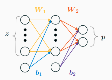
and the log-likelihood is, of course \[ \log p_{\boldsymbol{\mathbf{\theta}}}(\boldsymbol{\mathbf{x}}\mid \boldsymbol{\mathbf{z}}) = \sum_{j} x_j \log p_j + (1 - x_j) \log(1 - p_j) \]

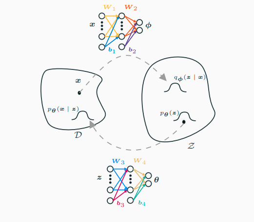
A Variational Autoencoder is simply Auto-Encoding Variational Bayes where both the approximating distribution \(q_{\boldsymbol{\mathbf{\phi}}}(\boldsymbol{\mathbf{z}}\mid \boldsymbol{\mathbf{x}})\) and \(p_{\boldsymbol{\mathbf{\theta}}}(\boldsymbol{\mathbf{x}}\mid\boldsymbol{\mathbf{z}})\) are parametrized using two different Neural Networks, as shown below.

Relationship between EM algorithm and VAE

So what is the relationship between the Expectation-Maximization algorithm and Variational Autoencoders? To get there we need to understand the EM algorithm in terms of Variational Inference. That is, we need to understand how the EM algorithm can be cast into the framework of variational inference. Recall that the EM algorithm proceeds in the following two steps:

• Compute “current” posterior (which we can call approximate since \(\boldsymbol{\mathbf{\theta}}^{(t)})\) will likely be, before convergence, different from the true \(\boldsymbol{\mathbf{\theta}}^*\)) \[ \displaystyle\left\{p_{\boldsymbol{\mathbf{\theta}}^{(t)}}(\boldsymbol{\mathbf{z}}\mid \boldsymbol{\mathbf{x}}) \,\, : \,\, \boldsymbol{\mathbf{x}}\in\mathcal{D}\right\} \]
• Find optimal parameter \[ \displaystyle \boldsymbol{\mathbf{\theta}}^{(t+1)} = \arg\max_{\boldsymbol{\mathbf{\theta}}} \sum_{\boldsymbol{\mathbf{x}}\in\mathcal{D}} \mathbb{E}_{p_{\boldsymbol{\mathbf{\theta}}^{(t)}}(\boldsymbol{\mathbf{z}}\mid \boldsymbol{\mathbf{x}})}\left[\log p_{\boldsymbol{\mathbf{\theta}}}(\boldsymbol{\mathbf{x}}, \boldsymbol{\mathbf{z}})\right] \]

Now consider the ELBO in its two different forms, but now rather than considering it as a function of \(\boldsymbol{\mathbf{x}}\) parametrized by \(\boldsymbol{\mathbf{\theta}}\) and \(\boldsymbol{\mathbf{\phi}}\) (i.e. \(\mathcal{L}_{\theta, \boldsymbol{\mathbf{\phi}}}(\boldsymbol{\mathbf{x}})\)), consider it as a functional of \(q_{\boldsymbol{\mathbf{\phi}}}\) and a function of \(\boldsymbol{\mathbf{\theta}}\), i.e. \(\mathcal{L}_{\boldsymbol{\mathbf{x}}}(\boldsymbol{\mathbf{\theta}}, q_{\boldsymbol{\mathbf{\phi}}})\).

\[\begin{equation*} \mathcal{L}_{\boldsymbol{\mathbf{x}}}(\boldsymbol{\mathbf{\theta}}, q_{\boldsymbol{\mathbf{\phi}}})= \begin{cases} \displaystyle \log p_{\boldsymbol{\mathbf{\theta}}}(\boldsymbol{\mathbf{x}})- \text{KL}(q_{\boldsymbol{\mathbf{\phi}}}\,\,||\,\,p_{\boldsymbol{\mathbf{\theta}}}(\boldsymbol{\mathbf{z}}\mid \boldsymbol{\mathbf{x}})) \qquad \qquad &(1)\\ \qquad \\ \displaystyle \mathbb{E}_{q_{\boldsymbol{\mathbf{\phi}}}}[\log p_{\boldsymbol{\mathbf{\theta}}}(\boldsymbol{\mathbf{x}}, \boldsymbol{\mathbf{z}})] - \mathbb{E}_{q_{\boldsymbol{\mathbf{\phi}}}}[\log q_{\boldsymbol{\mathbf{\phi}}}] \qquad \qquad &(2) \end{cases} \end{equation*}\]

We can find two identical steps as those of the EM algorithm by performing maximization of the ELBO with respect to \(q_{\boldsymbol{\mathbf{\phi}}}\) first, and then with respect to \(\boldsymbol{\mathbf{\theta}}\):

• E-step: Maximize \((1)\) with respect to \(q_{\boldsymbol{\mathbf{\phi}}}\) (this makes the KL-divergence zero and the bound is tight) \[ \left\{p_{\boldsymbol{\mathbf{\theta}}^{(t)}}(\boldsymbol{\mathbf{z}}\mid \boldsymbol{\mathbf{x}})= \arg\max_{q_{\boldsymbol{\mathbf{\phi}}}} \mathcal{L}_{\boldsymbol{\mathbf{x}}}(\boldsymbol{\mathbf{\theta}}^{(t)}, q_{\boldsymbol{\mathbf{\phi}}})\,\, : \,\, \boldsymbol{\mathbf{x}}\in\mathcal{D}\right\} \]
• M-step: Maximize \((2)\) with respect to \(\boldsymbol{\mathbf{\theta}}\) \[ \boldsymbol{\mathbf{\theta}}^{(t+1)} = \arg\max_{\boldsymbol{\mathbf{\theta}}} \sum_{\boldsymbol{\mathbf{x}}\in\mathcal{D}} \mathcal{L}_{\boldsymbol{\mathbf{x}}}(\boldsymbol{\mathbf{\theta}}, p_{\boldsymbol{\mathbf{\theta}}^{(t)}}(\boldsymbol{\mathbf{z}}\mid \boldsymbol{\mathbf{x}})) \]

The relationship between the Expectation Maximization algorithm and Variational Auto-Encoders can therefore be summarized as follows:

• EM algorithm and VAE optimize the same objective function.
• When expectations are in closed-form, one should use the EM algorithm which uses coordinate ascent.
• When expectations are intractable, VAE uses stochastic gradient ascent on an unbiased estimator of the objective function.