Minimalist Variational Autoencoder in Pytorch with CUDA GPU

Introduction to Variational Autoencoders (VAE) in Pytorch

Coding a Variational Autoencoder in Pytorch and leveraging the power of GPUs can be daunting. This is a minimalist, simple and reproducible example. We will work with the MNIST Dataset. The training set contains \(60\,000\) images, the test set contains only \(10\,000\). We will code the Variational Autoencoder (VAE) in Pytorch because it’s much simpler and yet flexible enough to code it in a few different ways. For this reason, in this post we will see the most minimalist version of a Variational Autoencoder, and then in the next post Assessing a Variational Autoencoder on MNIST using Pytorch we will see a slightly more verbose version that can be used for data generation and visualization of the Latent Space.

Download MNIST Dataset

Images in the MNIST Dataset are in grayscale, they are made of \(28\times 28\) pixels whose values range between \(0\) and \(255\). Notice that since its grayscale, we only have one number per pixel. In contrast, if the images where colored, then we would have \(3\) numbers per pixel, each one of them representing the intensity of Red, Green and Blue (RGB).

In Pytorch there’s a two-step process to use a dataset.

• Create a Dataset object. You can consider this as an abstract version of the dataset you want to work with. It has key informations such as its length and how to grab batches from it. By creating this Dataset object you download the data and prepare the groundwork for the Dataloader object.
• Create a Dataloader object. This is an object that you can iterate over and it will give you a batch of data and its corresponding labels.

Importantly, when defining the Dataset object, you can specify how to preprocess the data, e.g. scaling the data. In VAE we are assuming that each feature (i.e. each pixel value) can be interpreted as a probability. For this reason, we want to scale our pixel values to be in the range \([0, 1]\).

Notice that very often, when using other methods, people normalize the pixel values to be centered around zero and to have unit standard deviation. This must not be done in this case because we cannot have negative pixel values.

Here’s one way to load the MNIST dataset.

# Import libraries
import torchvision                             # contains image datasets and many functions to manipulate images
import torchvision.transforms as transforms    # to normalize, scale etc the dataset
from torch.utils.data import DataLoader        # to load data into batches (for SGD)
from torchvision.utils import make_grid        # Plotting. Makes a grid of tensors
from torchvision.datasets import MNIST         # the classic handwritten digits dataset
import matplotlib.pyplot as plt                # to plot our images
import numpy as np

# Create Dataset object.s Notice that ToTensor() transforms images to pytorch
# tensors AND scales the pixel values to be within [0, 1]. Also, we have separate Dataset
# objects for training and test sets. Data will be downloaded to a folder called 'data'.
trainset = MNIST(root='./data', train=True, download=True, transform=transforms.ToTensor())
testset  = MNIST(root='./data', train=False, download=True, transform=transforms.ToTensor())

# Create DataLoader objects. These will give us our batches of training and testing data.
batch_size = 100
trainloader = DataLoader(trainset, batch_size=batch_size, shuffle=True)
testloader  = DataLoader(testset, batch_size=batch_size, shuffle=True)

Set up CUDA GPU for faster training

If you have a GPU the following should print device(type='cuda', index=0).

import torch
device = torch.device("cuda:0" if torch.cuda.is_available() else "cpu")
print(device)

Variational Autoencoder in Pytorch

First, we import the necessary libraries.

import torch.nn as nn                          # Class that implements a model (such as a Neural Network)
import torch.nn.functional as F                # contains activation functions, sampling layers etc
import torch.optim as optim                    # For optimization routines such as SGD, ADAM, ADAGRAD, etc

Next, we define some global variables that are going to be used by our Variational AutoEncoder.

e_hidden = 500        # Number of hidden units in the encoder. See AEVB paper page 7, section "Marginal Likelihood"
d_hidden = 500        # Number of hidden units in the decoder. See AEVB paper page 7, section "Marginal Likelihood"
latent_dim = 2        # Dimension of latent space. See AEVB paper, page 7, section "Marginal Likelihood"
learning_rate = 0.001 # For optimizer (SGD or Adam)
weight_decay = 1e-5   # For optimizer (SGD or Adam)
epochs = 50           # Number of sweeps through the whole dataset

Finally, we can define the variational autoencoder. The simplest way to do so is to create a new class, which we call VAE inheriting from Pytorch’s nn.Module class. Essentially, all we need to do is to define a method called forward. This method should take one input parameter which corresponds to an image and it should output its reconstruction. It describes what happens to an image when it goes throught the Variational Autoencoder.

To simplify notation, we define some variables in the constructor __init__(). In particular, we define the set of operations that we are going to use in the forward() method.

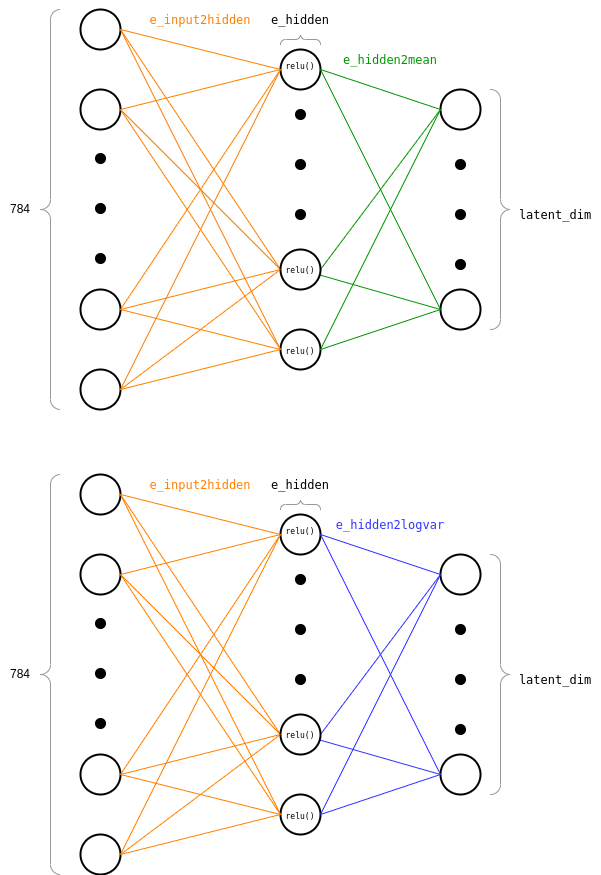
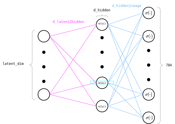
• self.e_input2hidden() is a function that takes an input image and feeds it through the first set of weights. These are the weights connecting the input layer to the hidden layer.
• self.e_hidden2mean() and self.e_hidden2logvar() are two functions that take the resulting activations in the hidden layer and feed them through two different sets of weights, connecting the hidden layer to a \(\mu\)-output layer and a \(\log\sigma^2\)-output layer. Basically together these represent all the parameters of the Encoder network. When we feed an image through the Variational Autoencoder, this goes through a feed-forward neural network with one hidden layer and 2 output layers. Each output layer has the same number of neurons, i.e. the dimension of the latent space, which is specified by latent_dim. One output layer gives us what will later be the mean of the latent space representation of that image and the other output layer gives us what will later be the log variance of the latent space representation of that image.
• self.d_latent2hidden() is a function that takes a latent representation z and feeds it through a first set of weights, connecting the latent space to the first hidden layer.
• self.d_hidden2image() is a function that takes the activations in such hidden layer and feeds them through a second set of weights, connecting the hidden layer to the image space. Essentially, these two functions represent the parameters of the Decoder which takes a latent representation and returns a flattened reconstructed image.

class VAE(nn.Module):
    def __init__(self):
        """Variational Auto-Encoder Class"""
        super(VAE, self).__init__()
        # Encoding Layers
        self.e_input2hidden = nn.Linear(in_features=784, out_features=e_hidden)
        self.e_hidden2mean = nn.Linear(in_features=e_hidden, out_features=latent_dim)
        self.e_hidden2logvar = nn.Linear(in_features=e_hidden, out_features=latent_dim)
        
        # Decoding Layers
        self.d_latent2hidden = nn.Linear(in_features=latent_dim, out_features=d_hidden)
        self.d_hidden2image = nn.Linear(in_features=d_hidden, out_features=784)
        
    def forward(self, x):
        # Shape Flatten image to [batch_size, input_features]
        x = x.view(-1, 784)
        
        # Feed x into Encoder to obtain mean and logvar
        x = F.relu(self.e_input2hidden(x))
        mu, logvar = self.e_hidden2mean(x), self.e_hidden2logvar(x)
        
        # Sample z from latent space using mu and logvar
        if self.training:
            z = torch.randn_like(mu).mul(torch.exp(0.5*logvar)).add_(mu)
        else:
            z = mu
        
        # Feed z into Decoder to obtain reconstructed image. Use Sigmoid as output activation (=probabilities)
        x_recon = torch.sigmoid(self.d_hidden2image(torch.relu(self.d_latent2hidden(z))))
        
        return x_recon, mu, logvar

As we can see above, the first operation in forward() is to make sure that the input is flattened. This is needed because it has to go through a feed-forward fully-connected layer (also called Linear in Pytorch). Notice that when I say that the input is flattened I don’t mean that it’s one dimensional. Rather, we are flattening the height and the width of the image into one dimension.

The input to the Variational AutoEncoder will need to be shaped [batch_size, input_features]. Unfortunately, when we iterate over the DataLoader, we get an object that is shaped [batch_size, channels, height, width]. In our case, since we have only one color channel and images are 28x28 this means that we get [batch_size, 1, 28, 28]. To feed this batch of images to the Variational Autoencoder we simply flatten the last \(3\) dimensions so that each pixel value of each channel is a feature. That is, we shape it to be [batch_size, 784]. In the code above, I’ve used x.view(-1, 784) and, similarly to Numpy, this means that we want the second dimension to be 784 and we let Pytorch work out what the second dimension will be (in this case 100).

Then, we feed the batch images of size [batch_size, 784] onto our first set of weights and we feed this into a Rectified Linear Unit activation function. At this point our batch of images has shape [batch_size, e_hidden]. Then we feed these activations through two different output layers, thus obtaining our latent mu and logvar. The output of each of these layers has shape [batch_size, latent_dim].

Then, during training, we sample from a Normal distribution with that mean and variance. In order to allow backpropagation to flow through the network, we need to use the reparametrization trick. This simply consists in first sampling from a standard normal distribution (with shape [batch_size, latent_dim]), scaling it by the standard deviation and adding the mean to it. If we are not training the network anymore, we simply output mu so that the output is reproducible every time (which also has shape [batch_size, latent_dim]).

Finally, we take the sampled latent representation, we feed it through a first set of weights, through a Relu activation function (so its shape is not [batch_size, d_hidden]), through a second set of weights (connecting the hidden layer to the output layeter), and finally we feed this through a Sigmoid activation function (so that the final shape is [batch_size, 784]). We use sigmoid activation function because, as you can remember from the previous Variational Autoencoders post, each of our pixels is considered a probability, so we need our output to be between [0, 1].

Below is an example of what the encoder looks like:

And similarly, what the decoder looks like:

Pytorch VAE Training

We are now ready to train the Variational Autoencoder.First, we define our loss. Remember that maximizing the evidence can be approximately done by maximizing the ELBO (Evidence Lower Bound) which can be written as a difference of two terms:

\[ \mathcal{L}_{\theta, \boldsymbol{\mathbf{\phi}}}(\boldsymbol{\mathbf{x}})= \underbrace{\mathbb{E}_{q_{\boldsymbol{\mathbf{\phi}}}}\left[\log p_{\boldsymbol{\mathbf{\theta}}}(\boldsymbol{\mathbf{x}}\mid \boldsymbol{\mathbf{z}})\right]}_{\text{Expected Log-Likelihood}} - \underbrace{\text{KL}(q_{\boldsymbol{\mathbf{\phi}}}(\boldsymbol{\mathbf{z}}\mid \boldsymbol{\mathbf{x}})\,\,||\,\,p_{\boldsymbol{\mathbf{\theta}}}(\boldsymbol{\mathbf{z}}))}_{\text{Regularization Term}} \]

In the case of both \(q_{\boldsymbol{\mathbf{\phi}}}\) and \(q_{\boldsymbol{\mathbf{\phi}}}(\boldsymbol{\mathbf{z}}\mid \boldsymbol{\mathbf{x}})\) being Gaussians the AEVB paper shows that the following formula is available

\[ -\text{KL}(q_{\boldsymbol{\mathbf{\phi}}}\,\,||\,\,q_{\boldsymbol{\mathbf{\phi}}}(\boldsymbol{\mathbf{z}}\mid \boldsymbol{\mathbf{x}})) = \frac{1}{2}\sum_{j=1}^J \left[1 + \log\sigma_j^2 - \mu_j^2 - \sigma_j^2\right] \] where \(J\) is the dimensionality of \(\boldsymbol{\mathbf{z}}\) which, in our case, is denoted latent_dim.

Then an unbiased estimate for the Objective is given below:

\[ \widetilde{\mathcal{L}}_{\boldsymbol{\mathbf{\theta}}, \boldsymbol{\mathbf{\phi}}}(\boldsymbol{\mathbf{x}}) = \displaystyle \frac{1}{L}\sum_{i=1}^L \left[\log p_{\boldsymbol{\mathbf{\theta}}}(\boldsymbol{\mathbf{x}}\mid g_{\boldsymbol{\mathbf{\phi}}}(\boldsymbol{\mathbf{\epsilon}}^{(i)}, \boldsymbol{\mathbf{x}}))\right] - \frac{1}{2}\sum_{j=1}^J \left[1 + \log\sigma_j^2 - \mu_j^2 - \sigma_j^2\right] \qquad \text{where } \boldsymbol{\mathbf{\epsilon}}^{(i)} \overset{\text{i.i.d.}}{\sim}\mathcal{N}(\boldsymbol{\mathbf{0}}, \boldsymbol{\mathbf{I}}) \]

Where \(L=\) L and \(J=\) latent_dim.

Recall that in the case of Bernoulli variables the log-likelihood becomes

\[ \log p_{\boldsymbol{\mathbf{\theta}}}(\boldsymbol{\mathbf{x}}\mid \boldsymbol{\mathbf{z}}) = \sum_{j} x_j \log p_j + (1 - x_j) \log(1 - p_j) \] Since we want our pixel values to be between 0 and 1 this is exactly what we are looking for and thankfully is already implemented in Pytorch under the name of binary_crossentropy.

# Loss
def vae_loss(image, reconstruction, mu, logvar):
  """Loss for the Variational AutoEncoder."""
  # Binary Cross Entropy for batch
  BCE = F.binary_cross_entropy(input=reconstruction.view(-1, 28*28), target=image.view(-1, 28*28), reduction='sum')
  # Closed-form KL Divergence
  KLD = 0.5 * torch.sum(1 + logvar - mu.pow(2) - logvar.exp())
  return BCE - KLD

# Instantiate VAE with Adam optimizer
vae = VAE()
vae = vae.to(device)    # send weights to GPU. Do this BEFORE defining Optimizer
optimizer = optim.Adam(params=vae.parameters(), lr=learning_rate, weight_decay=weight_decay)
vae.train()            # tell the network to be in training mode. Useful to activate Dropout layers & other stuff

# Train
losses = []

for epoch in range(epochs):
  # Store training losses & instantiate batch counter
  losses.append(0)
  number_of_batches = 0

  # Grab the batch, we are only interested in images not on their labels
  for images, _ in trainloader:
    # Save batch to GPU, remove existing gradients from previous iterations
    images = images.to(device)
    optimizer.zero_grad()

    # Feed images to VAE. Compute Loss.
    reconstructions, latent_mu, latent_logvar = vae(images)
    loss = vae_loss(images, reconstructions, latent_mu, latent_logvar)

    # Backpropagate the loss & perform optimization step with such gradients
    loss.backward()
    optimizer.step()

    # Add loss to the cumulative sum
    losses[-1] += loss.item()  
    number_of_batches += 1
  
  # Update average loss & Log information
  losses[-1] /= number_of_batches
  print('Epoch [%d / %d] average reconstruction error: %f' % (epoch+1, epochs, losses[-1]))    

You should see an output similar to the following:

Epoch [1 / 10] average reconstruction error: 18439.412160
Epoch [2 / 10] average reconstruction error: 16523.078558
Epoch [3 / 10] average reconstruction error: 16100.590828
Epoch [4 / 10] average reconstruction error: 15850.990076
Epoch [5 / 10] average reconstruction error: 15673.100459
Epoch [6 / 10] average reconstruction error: 15539.618418
Epoch [7 / 10] average reconstruction error: 15431.895505
Epoch [8 / 10] average reconstruction error: 15348.046214
Epoch [9 / 10] average reconstruction error: 15278.517415
Epoch [10 / 10] average reconstruction error: 15210.919212

To learn how you can test the Variational Autoencoder, how to use it to generate data and how to visualize the latent space have a look at my new blog post: Assessing a Variational Autoencoder on MNIST using Pytorch.

You can find the code in this blogpost in this Google Colab notebook.