Gaussian with Unknown Variance and Unknown Mean

Finding the Objective Function

Suppose that now we want to generate samples from $\mathcal{N}(\mu ,\sigma )$ rather than $\mathcal{N}(\mu ,1)$. This makes the calculations a bit more involved than in the previous example because now also $\sigma$ is unknown, but the general idea is the same.

Once again, we find the expression for $p(x)$ using the change of variable formula. This time the transformation is $$g(z)=\sigma z+\mu$$ leading to $$p(g^{-1}(x))=-\frac{1}{2}\log (2\pi )-\frac{(x-\mu {)}^2}{2{\sigma }^2}.$$ Since ${\partial }_x{g}^{-1}(x)={\sigma }^{-1}$ we get $$\log p(x)=-\frac{1}{2}\log (2\pi )-\frac{(x-\mu {)}^2}{2{\sigma }^2}-\log \sigma .$$

The average log-likelihood is then given by the following expression: $$\frac{1}{n}\sum _{i=1}^n\log p(x^{(i)})=-\frac{1}{2}\log (2\pi )-\frac{1}{2n{\sigma }^2}\sum _{i=1}^n(x^{(i)}-\mu {)}^2-\log \sigma$$

Gradient Estimates and Updates

Firstly, we take the derivative with respect to $\mu$: $$\frac{\partial }{\partial \mu }\frac{1}{n}\sum _{i=1}^n\log p(x^{(i)})=\frac{1}{n{\sigma }^2}\sum _{i=1}^n(x_i-\mu )=\frac{\bar{x}}{{\sigma }^2}-\frac{\mu }{{\sigma }^2}$$

Similarly, the derivative with respect to $\sigma$ is given by $$\frac{\partial }{\partial \sigma }\frac{1}{n}\sum _{i=1}^n\log p(x^{(i)})=\frac{1}{n{\sigma }^3}\sum _{i=1}^n(x^{(i)}-\mu {)}^2-\frac{1}{\sigma }$$

This means that our updates will be $$\begin{array}{rl}{\mu }_{t+1}& ⟵{\mu }_t+{\gamma }_{\mu }(\frac{\bar{x}}{{\sigma }_t^2}-\frac{{\mu }_t}{{\sigma }_t^2})\\ {\sigma }_{t+1}& ⟵{\sigma }_t+{\gamma }_{\sigma }(\frac{1}{n{\sigma }_t^3}\sum _{i=1}^n(x^{(i)}-{\mu }_{t+1}{)}^2-\frac{1}{{\sigma }_t})\end{array}$$

where ${\gamma }_{\mu }$ and ${\gamma }_{\sigma }$ represent the (possibly) different step sizes for $\mu$ and $\sigma$ respectively.

Coding

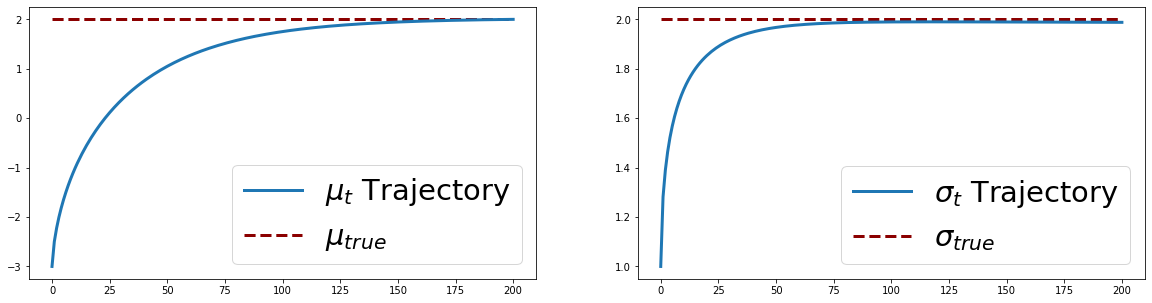
The code below is very similar to the one for example 1. The only differences are that now we have both a true $\mu$ and a true $\sigma$. In this example, we’ve fixed them at ${\mu }_{\text{true}}=2.0$ and ${\sigma }_{\text{true}}=2.0$. We start with guesses $-3.0$ and $1.0$ for $\mu$ and $\sigma$ respectively. Notice how we use two different step sizes for ${\mu }_t$ and ${\sigma }_t$.

# Import stuff
import math
import numpy as np
import matplotlib.pyplot as plt
import scipy.stats as stats

# Generate data
n = 10000
mu_true = 2.0
sigma_true = 2.0
x = np.random.normal(loc=mu_true, scale=sigma_true, size=n)

# Algorithm Settings
mu = -3.0        # Start with mu = -1.0
sigma = 1.0      # Start with sigma = 1.0
gamma_mu = 0.1      # Learning rate
gamma_sigma = 0.01
n_iter = 500     # Number of iterations

# Loop through and update mu and sigma
mus = [mu]
sigmas = [sigma]
for i in range(n_iter):
    # Compute gradients
    mu_grad = (np.mean(x) - mu) / (sigma**2)
    sigma_grad = (np.mean((x - mu)**2)/sigma**3 - 1 / sigma)
    # Update mu and sigma
    mu, sigma = mu + gamma_mu*mu_grad, sigma + gamma_sigma*sigma_grad
    # Store mu and sigma
    mus.append(mu)
    sigmas.append(sigma)
    
fig, ax = plt.subplots(nrows=1, ncols=2, figsize=(20, 5))
# Plot mu trajectory
ax[0].plot(range(n_iter+1), mus, lw=3)
ax[0].hlines(y=mu_true, xmin=0, xmax=n_iter, 
          color='darkred', linestyle='dashed', lw=3)
ax[0].legend([r'$\mu_t$' + " Trajectory", r'$\mu_{true}$'], prop={'size': 29}, loc='lower right')
# Plot sigma trajectory 
ax[1].plot(range(n_iter+1), sigmas, lw=3)
ax[1].hlines(y=sigma_true, xmin=0, xmax=n_iter, 
          color='darkred', linestyle='dashed', lw=3)
ax[1].legend([r'$\sigma_t$' + " Trajectory", r'$\sigma_{true}$'], prop={'size': 29})
plt.show()

You can find and run a working version of this Google Colab notebook. .