Towards SMC: Using the Dirac-delta function in Sampling and Sequential Monte Carlo

Discrete Distributions, PMF and CDF

Suppose we have a discrete random variable \(X\) taking \(k\) different values \[ \mathbb{P}[X = x_i] = p_i \qquad \forall\, i = 1, \ldots, k, \] where \(0\leq p_i \leq 1\) and \(\sum_{i=1}^k p_i = 1\). It’s probability mass function is then equal to \(p_i\) at \(X=x_i\) and \(0\) everywhere else, as shown in Figure 1 \[ P_X(x) = \begin{cases} p_i & x=x_i \\ 0 & x\neq \{x_1, \ldots, x_k\} \end{cases}. \]

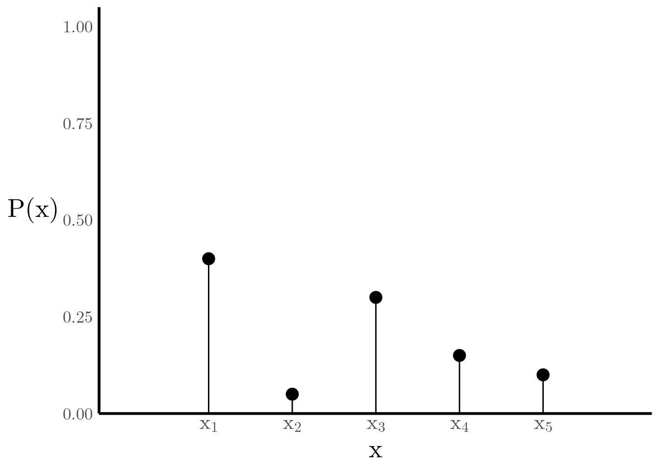
Figure 1: Probability Mass Function

The cumulative distribution function of \(X\), denoted \(F_X(x)\), gives us the probability that the state of \(X\) is less than or equal to \(x\) (see Figure 2) \[ F_X(x) = \sum_{x_i \leq x} \mathbb{P}[X = x_i] \qquad\qquad -\infty < x < \infty. \]

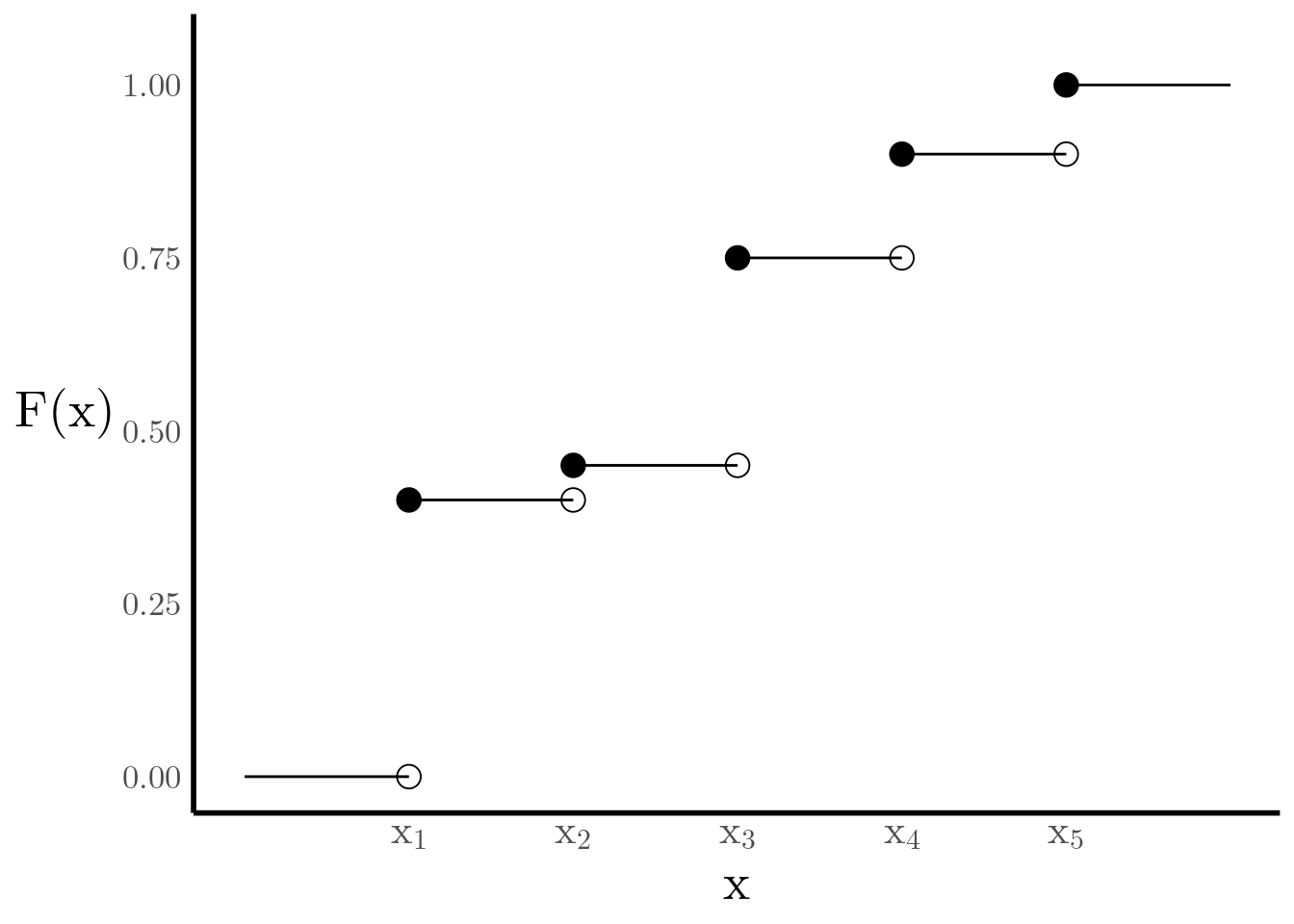
Figure 2: Cumulative Distribution Function

Rewriting Discrete Distributions as Continuous Distributions

We can also express the CDF as a sum of step functions. For this purpose we define \(u_y(x)\) \[ u_{y}(x) = \begin{cases} 1 & x\geq y \\ 0 & x < y \end{cases}, \]

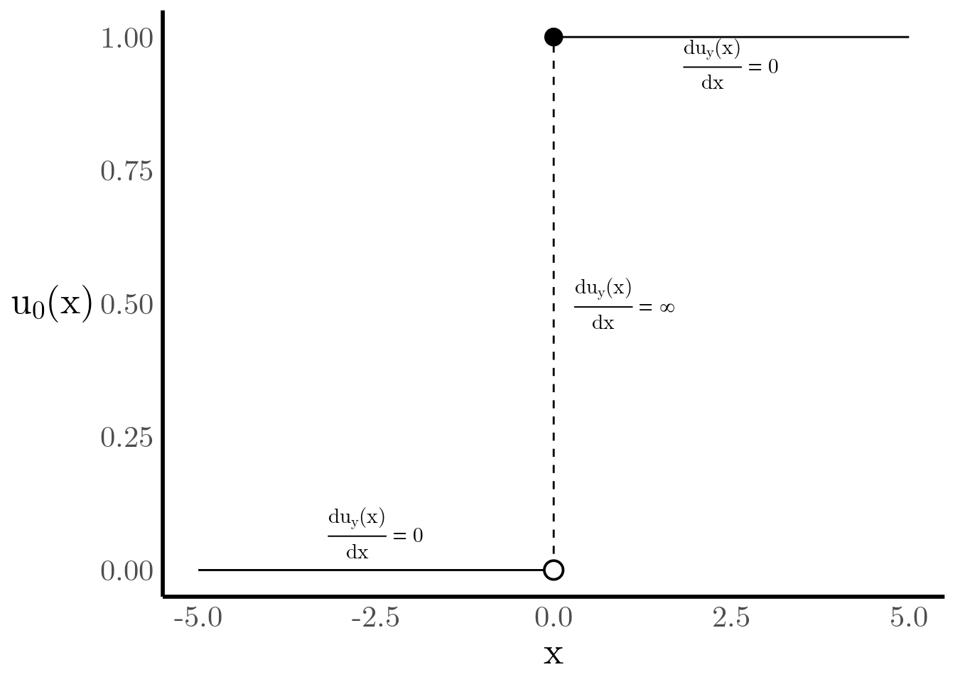
Figure 3: Step Function

and then rewrite the CDF as follows \[ F_X(x) = \sum_{i=1}^N \mathbb{P}\left(X = x_i\right) u_{x^{(i)}}(x) = \sum_{i=1}^N p_i u_{x^{(i)}}(x) \] This way of writing the CDF is more useful because, if we can find a suitable derivative for the step function, then we can find an approximation to the PDF. Unfortunately, the step function has a discontinuity at \(x=y\). The solution to this problem lies in defining the derivative of the step function ourselves. We call this the Dirac Delta function and it satisfies the following properties (for any function \(g(x)\)) \[ \frac{d \,u_{y}(x)}{d x} = \delta_y(x) = \begin{cases} \infty & x=y \\ 0 & x\neq y \end{cases} \] \[ \int g(x) \delta_y(x) dx = g(y) \]

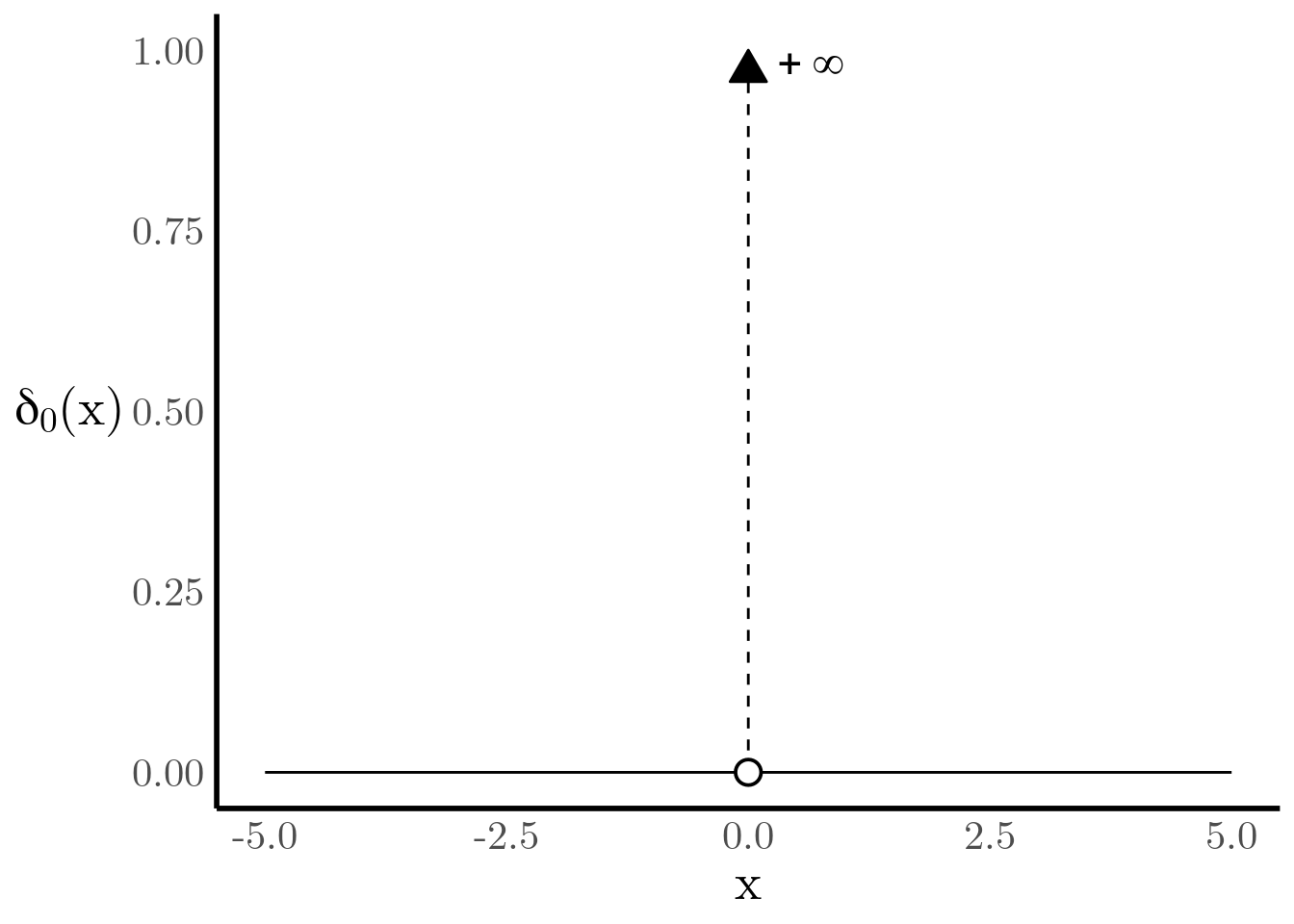
Figure 4: Dirac-delta Function

Now we can find an approximate continuous PDF for \(X\) by taking the derivative of \(F_X(x)\) \[ p_X(x) = \frac{d F_X(x)}{dx} = \sum_{i=1}^Np_i \frac{d u_{x^{(i)}}(x)}{dx} = \sum_{i=1}^Np_i \delta_{x^{(i)}}(x) \]

##Continuous approximation of an Empirical PDF Suppose now that we obtain realizations \(x^{(1)}, \ldots, x^{(N)}\) of a sample \(X^{(1)}, \ldots, X^{(N)}\) from a probability density function \(p_X(x)\). Since we only have a finite number \(N\) of such samples, we need to find a way of obtaining an approximate representation of \(p_X(x)\) from them. One step towards this goal is to construct the empirical distribution function \[ \widehat{F}_N(x) = \frac{1}{N}\sum_{i=1}^N \mathbb{I}(X^{(i)} \leq x) = \sum_{i=1}^N\frac{1}{N} \mathbb{I}(X^{(i)} \leq x), \] which essentially uses the indicator function to count how many observations of the sample are less than or equal to \(x\) and then divides it by \(N\), the number of samples. Another way of interpreting it is that is assigns probability \(\frac{1}{N}\) to each sample. Practically, this means that \(\widehat{F}_N(x)\) will be conceptually similar to Figure 2, but with jumps of \(\frac{1}{N}\) at every sample.

For instance, suppose that we sample \(N=5\) times from a standard normal \(\mathcal{N}(0, 1)\) and we sort the samples in increasing order, as shown in Figure 5.

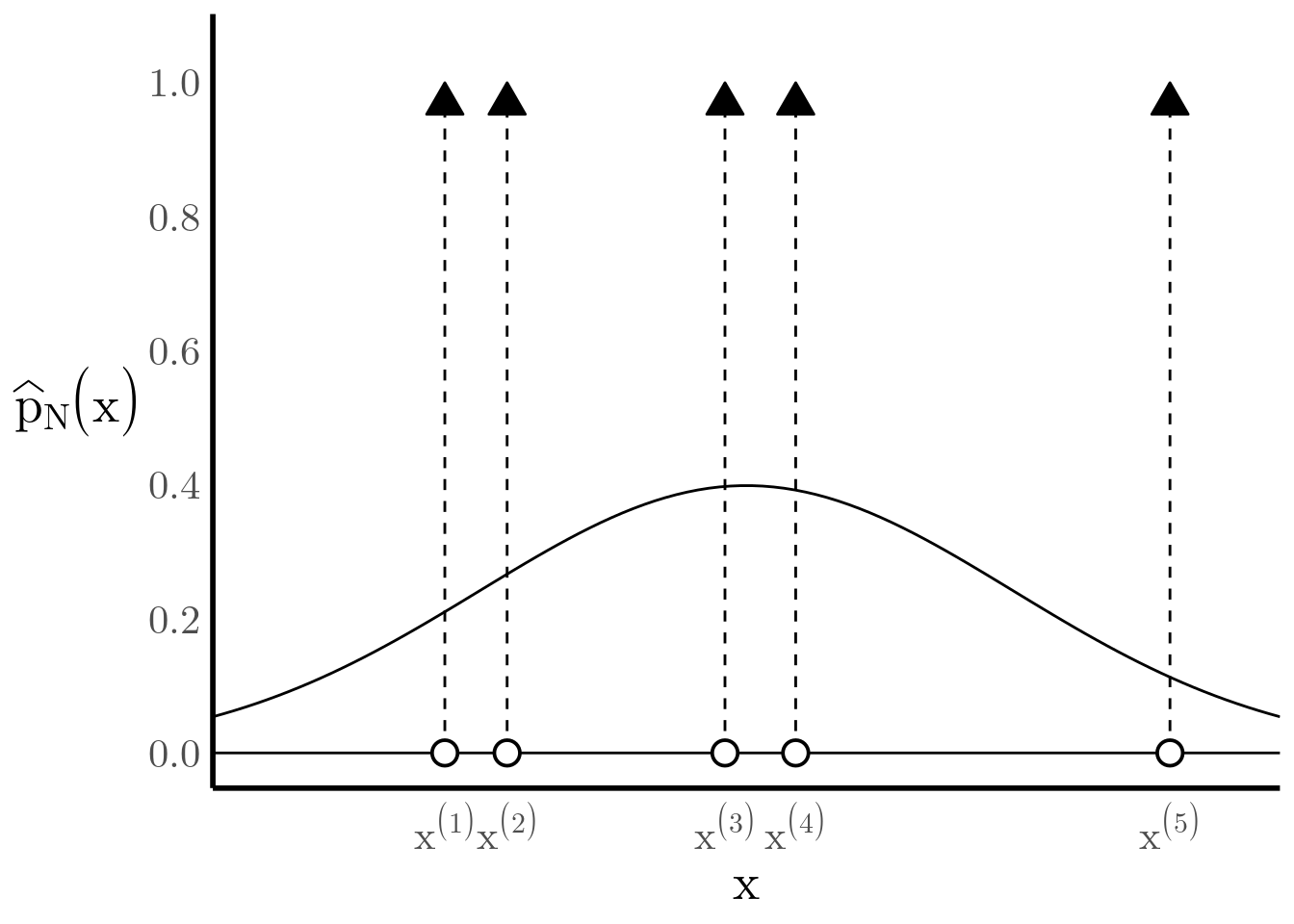
Figure 5: The true PDF \(\mathcal{N}\left(0, 1\right)\) is being approximated by a weighted sum of Dirac-delta functions.

We can build a CDF with jumps of \(\frac{1}{5}\) at every sample \(x^{(i)}\) (see Figure 6), and we can see how it gives a decent approximation of the true CDF. Importantly, by the Glivenko-Cantelli theorem we know that the empirical CDF converges to the true CDF as \(N\) increases.

Figure 6: he true CDF can be approximated by a weighted sum of step functions.

At this point, we can follow the same steps as above: rewrite the empirical CDF as a weighted sum of step functions, and then take the derivative to find an approximate PDF using the Dirac-delta function. \[ \widehat{F}_N(x) = \sum_{i=1}^{N} \frac{1}{N} u_{x^{(i)}}(x) \quad \implies \quad \widehat{p}_N(x) = \sum_{i=1}^{N} \frac{1}{N} \delta_{x^{(i)}}(x) \]