Reinforcement Learning from Human Feedback
Reinforcement Learning from Human Feedback (RLHF) was introduced in the InstructGPT paper. Suppose that $\pi_\theta$ is the distribution learned by a language model after Unsupervised Pre-Training (UPT) and Supervised Fine-Tuning (SFT), that is $$ \pi_\theta(x) = \text{Categorical}\left(\text{softmax}\left(\text{LLM}_{\theta}(x)\right)\right). $$ We would like to align our model to human preferences (or rather, contracted human labelers). RLHF frames this task as reinforcement learning.
Reinforcement Learning Recap
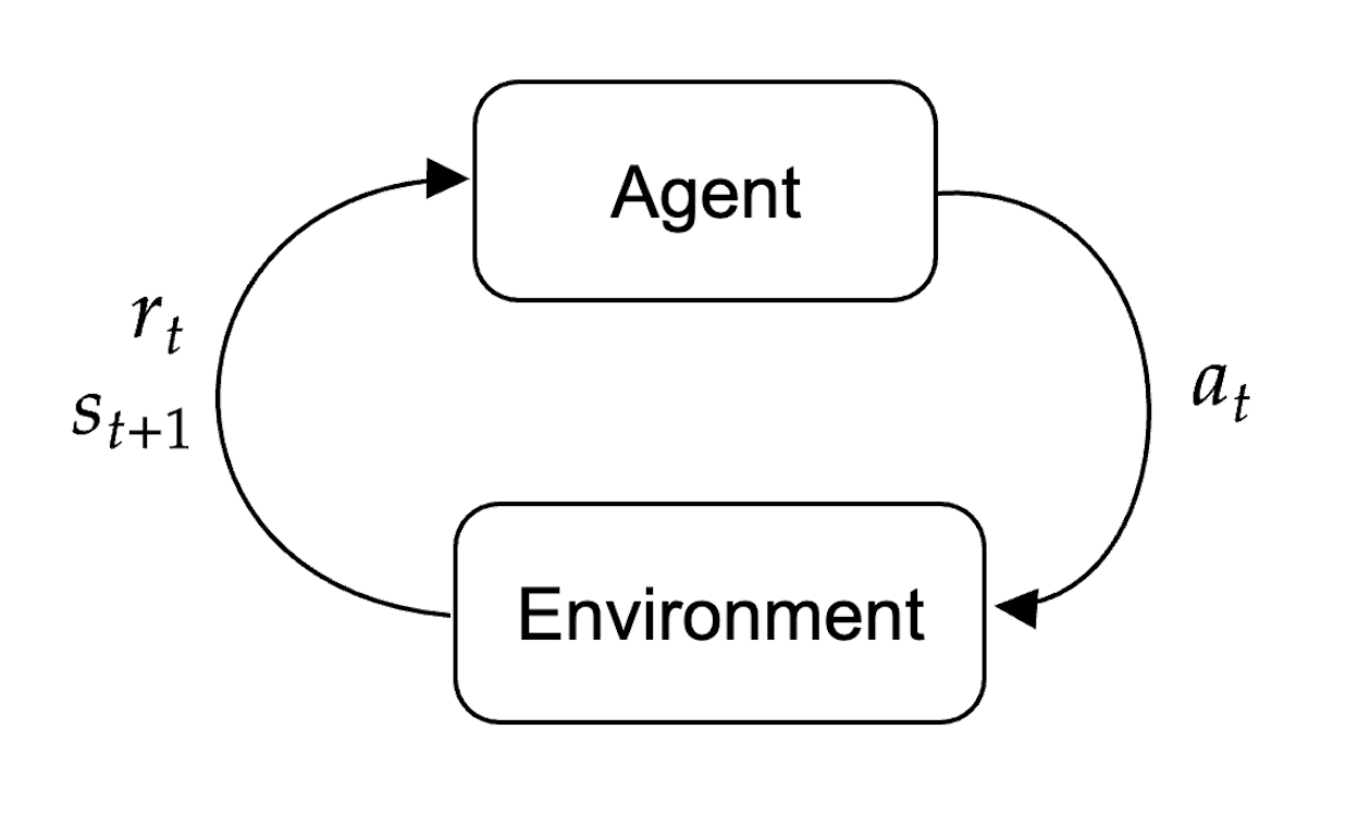
Reinforcement learning works as follows. In an environment with state $s_t$ there is an agent that can take actions $a_t$ in this environment according to a distribution $\pi_\theta(a_t\mid s_t)$, known as policy. After the agent performs an action, the environment then returns to the agent a state after the action $s_{t+1}$ and a reward $r_t$.
The aim is to learn a policy such that the expected reward is maximized $$ \max_{\theta} \,\,\mathbb{E}_{\pi_\theta(a_t\mid s_t)}[R(S_t)] $$ As we will see later, in the case of Language Modelling:
- Agent: Pre-trained and fine-tuned Language model
- State: Prompt
- Policy: Next-token distribution given the prompt
- Next-state: Sample from the categorical distribution represented by the LM
Baseline, Policy and Reward Models
We take our SF-tuned language model $\pi_{\theta}$ and create three identical copies:
- Baseline $\pi_0$: will have frozen parameters $\theta$ (unchanged through the entire RLHF process).
- Policy $\pi_\theta$: Will end up being our aligned model, we change its parameters during RLHF.
- Reward Model $r_\phi$: We copy $\pi_\theta$ a modification: we replace the last un-embedding layer: at the end of $\text{LLM}_\theta$ it will have one last linear layer that maps from $\mathbb{R}^{n_{emb}}$ to $\mathbb{R}^{n_{\text{vocab}}}$ so that we have one logit per token in the dictionary. This final linear layer is removed and replaced with a linear layer that maps $\mathbb{R}^{n_{emb}}$ to $\mathbb{R}$: we want a scalar reward. We call all of its parameters $\phi$.
However, in the original InstructGPT paper they said that for $r_\phi$ they used the same architecture as $\text{LLM}_\theta$, except that they made it much smaller ($6B$ parameters compared to $175B$). This is because it allows for faster reward modelling training and because using a larger reward model proved unstable.
Dataset of Human Preferences
For the next step, we focus exclusively on $r_\phi$. To generate a dataset of human preferences $\mathcal{D}_{\text{preferences}}$ we follow these steps
- For each prompt of interest $x_n$, sample $K$ from the policy $$ y_{n, 1}, \ldots, y_{n, K} \sim \pi_{\theta}(\cdot\mid x_n) $$
- Ask human labelers to rank all the resulting pairs of outputs (notice that there are ${K}\choose{2}$ pairs for each $x_n$). For each pair $(y_{n, k}, y_{n, j})$, $k\neq j$, the preferred output is now labelled $y_{n, w}$ and the not-preferred output is labelled $y_{n, l}$ where “w” and “l” stand for “winner” and “loser”. Mathematically, we write $y_{n, w} \succ y_{n, l}$.
This gives us the following human preferences dataset $$ \mathcal{D}_{\text{preferences}} = \left\{(x_n, y_{n, w}, y_{n, l})\,:\, n=1, \ldots, n_{\text{preferences}}\right\} $$
Training the Reward Model
The reward model will take pairs $(x, y)$ of prompt and target and return a scalar reward $r_\phi(x, y)$. We would like to train the parameters $\phi$. How do we train $r_\phi$? One option is to use the Bradley-Terry (BT) model, which assumes that the preferences in the dataset were generated by a true latent reward model $r^*(x, y)$ and that the preference distribution is $$ p^*(y_w \succ y_l \mid x) = \text{sigmoid}\left(r^*(x, y_w) - r^*(x, y_l)\right) $$ The higher this difference in reward, the higher the preference probability. This fundamentally transforms the problem into a binary classification problem between the class preferable and the class non-preferable. Therefore an obvious choice is to train $r_\phi$ by binary cross-entropy (or equivalently, maximum likelihood). The loss (negative log likelihood) is then $$ \mathcal{L}_{\text{RM}}(\phi) = -\mathbb{E}_{(x, y_w, y_l)\sim \mathcal{D}_{\text{preferences}}}\left[\log\left(\text{sigmoid}\left(r_\phi(x, y_w) - r_\phi(x, y_l)\right)\right)\right]. $$ As usual, we compute batched gradients however, the authors of InstructGPT suggest that to avoid overfitting during training, one should gather together all the comparisons from the same prompt into the same batch and perform a single forward pass of learning for the reward model.
Notice that the preference distribution (and so the loss) depends on the difference between the winning reward and the losing reward and it is therefore shift-invariant. After the reward model has been trained, the authors compute the average reward $\hat{r}$ across all human rankings and add a bias to the reward model (basically, they subtract this mean reward) so that the expected value of the reward is zero $$ \mathbb{E}_{(x, y)\sim\mathcal{D}_{\text{preferences}}}\left[r_\phi(X, Y)\right] = 0. $$
Reinforcement Learning
Now that we have available a reward model, we can use reinforcement learning to change the parameters of our policy $\pi_\theta$. We will see PPO and DPO.