Sample Space

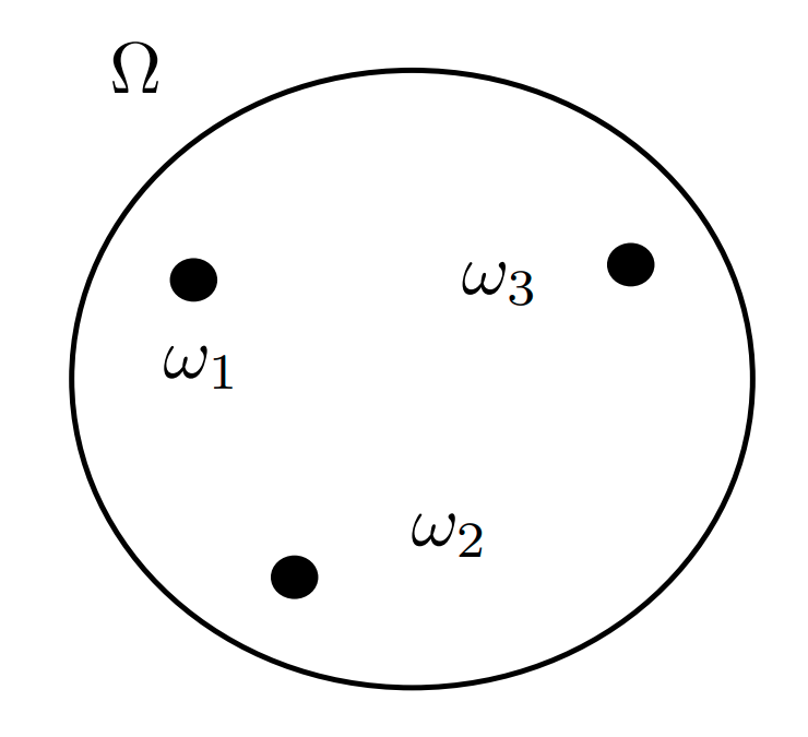
The sample space \(\Omega\) is the set of all outcomes of our probabilistic experiment.

For instance:

• Experiment: A single toss of a coin.
• Possible Outcomes: \(\omega_1 = \text{Head}\) and \(\omega_2 = \text{Tail}\).
• Sample Space: \(\Omega := \{\omega_1, \omega_2\} = \{\text{Head}, \text{Tail}\}\)

Event Space

The event space is a sigma-algebra on the sample space. It is a subset of the power set of \(\Omega\) whose elements, called events, satisfy some regularity conditions. When \(\Omega\) is finite and discrete, the power set \(\mathcal{P}(\Omega)\) is a valid sigma algebra that can be used as the event space.

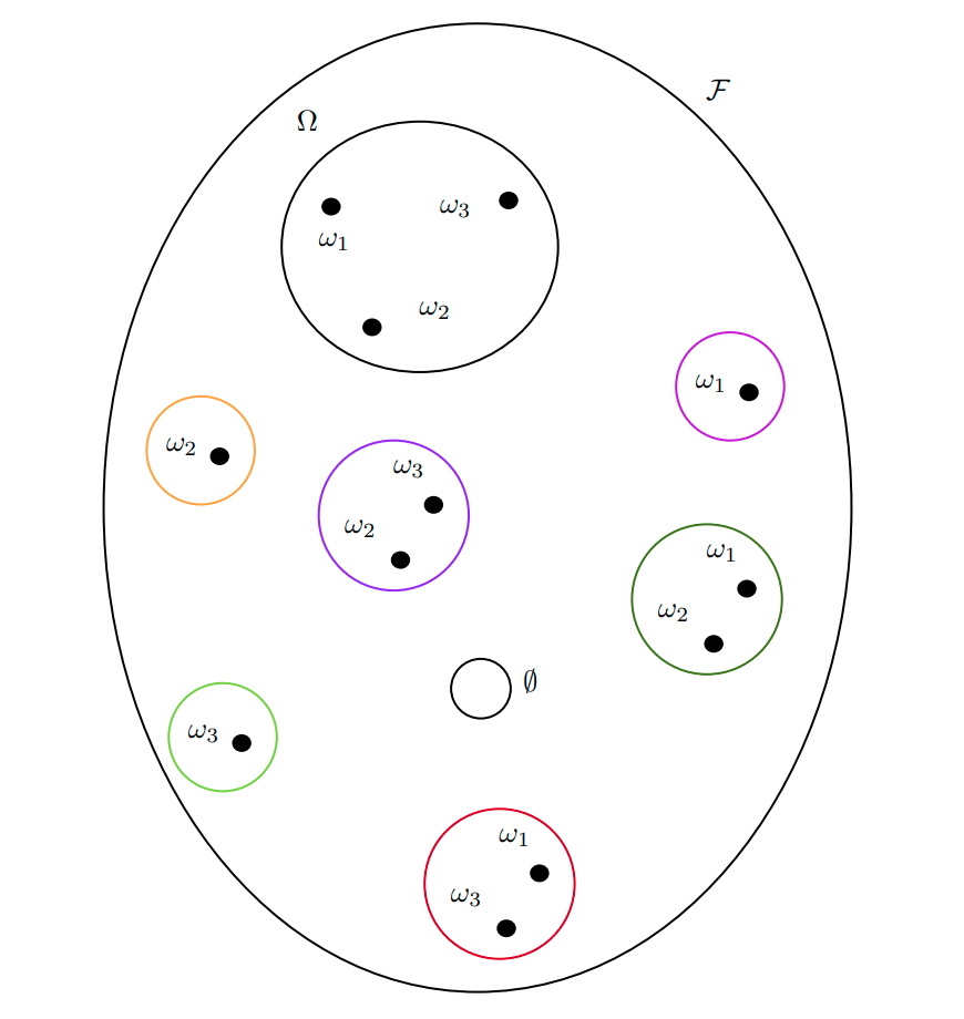
Practically \(\mathcal{F}\subseteq \mathcal{P}(\Omega)\) satisfying

• \(\Omega \in \mathcal{F}\) The sample space is an event (called the “sure” event).
• \(A\in \mathcal{F} \quad \implies \quad A^c\in\mathcal{F}\) Closed under complementation.
• \(A_1, A_2, \ldots\in\mathcal{F} \quad \implies \quad \cup_iA_i \in \mathcal{F}\) Closed under countable unions.

A pair \((\Omega, \mathcal{F})\) of a set and its sigma algebra (in this case of the sample space and the event space) is called a measurable space. This is because we can define a function that “measures” the size of the elements of all the elements of \(\mathcal{F}\). Indeed, any element of a sigma algebra \(B\in\mathcal{F}\) is called a measurable set.

Probability Measure and Probability Space

After you’ve defined the sigma-algebra called Event Space, the next step is to define a probability space. A probability space is a triplet \((\Omega, \mathcal{F}, \mathbb{P})\), i.e. it is composed of three elements, two of which we already know.

• A sample space \(\Omega\).
• An event space \(\mathcal{F}\) which is a sigma-algebra on \(\Omega\).
• A probability measure \(\mathbb{P}\).

A probability measure is a special case of a measure. Suppose you have a measurable space \((\Omega, \mathcal{F})\) (also referred to as \(\Omega\times\mathcal{F})\)). Then a function \[ \mathbb{P}: \mathcal{F} \to [0, +\infty) \] is called a measure on \((\Omega, \mathcal{F})\) if it gives a size of zero to the empty set and if it is countably additive:

• \(\mathbb{P}(\emptyset) = 0\)
• \(\mathbb{P}\left(\bigcup_i A_i\right) = \sum_i \mathbb{P}(A_i) \qquad \text{for } A_i\in\mathcal{F}\)

Notice how the measure takes elements of \(\mathcal{F}\) and not elements of the sample space! That is, it maps events not outcomes. A probability measure is just a measure, as above, with the additional property that it maps to \([0, 1]\) rather than to \([0, +\infty)\). In order words, it assigns probabilities to events, hence the name.

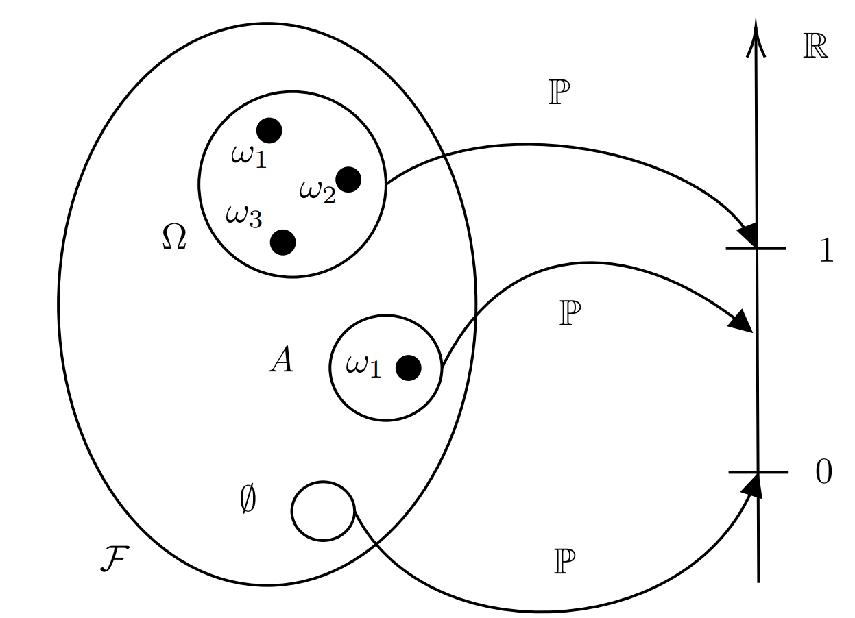
We can see in the diagram above how the probability measure maps the empty set to zero, the sample space to \(1\) and any other event to some number in \([0, 1]\).

Random Variable

A random variable is also called a measurable function. Suppose you have two measurable spaces. One could be the pair of sample space and event space \((\Omega, \mathcal{F})\), and the other one could be some other arbitrary pair of a set and of its sigma algebra \((\mathsf{E}, \mathcal{E})\), although usually we choose \(\mathsf{E} = \mathbb{R}\) and \(\mathcal{E} = \mathcal{B}(\mathbb{R})\). Then a measurable function is a function that maps elements in \(\Omega\) to elements in \(\mathsf{E}\) with some additional properties. Notice how this function maps outcomes to elements of \(\mathsf{E}\), it does not map events.

What property should this map satisfy? Imagine that we knew our sample space and event space, as in the coin tossing example. It might be a bit unhelpful to work on the actual sample space and event space, so instead we map them to alternative ones, that we are more comfortable using. For instance \(\mathbb{R}\) and \(\mathcal{B}(\mathbb{R})\). Then, it’s clear that we want our mapping to have a property that can guarantee us a sort of correspondence between the events in our original event space \(\mathcal{F}\) and our transformed event space \(\mathcal{E}\). For this reason, we require our measureable function, or random variable \[ X: \Omega \to \mathsf{E} \] to be such that the preimage \(X^{-1}(B)\) of any \(\mathcal{E}\)-measurable set \(B\in\mathcal{E}\) is a \(\mathcal{F}\)-measurable set. \[ X^{-1}(B) = \{\omega\in \Omega \, :\, X(\omega) \in B \} \in \mathcal{F} \qquad \forall \, B \in \mathcal{E} \]

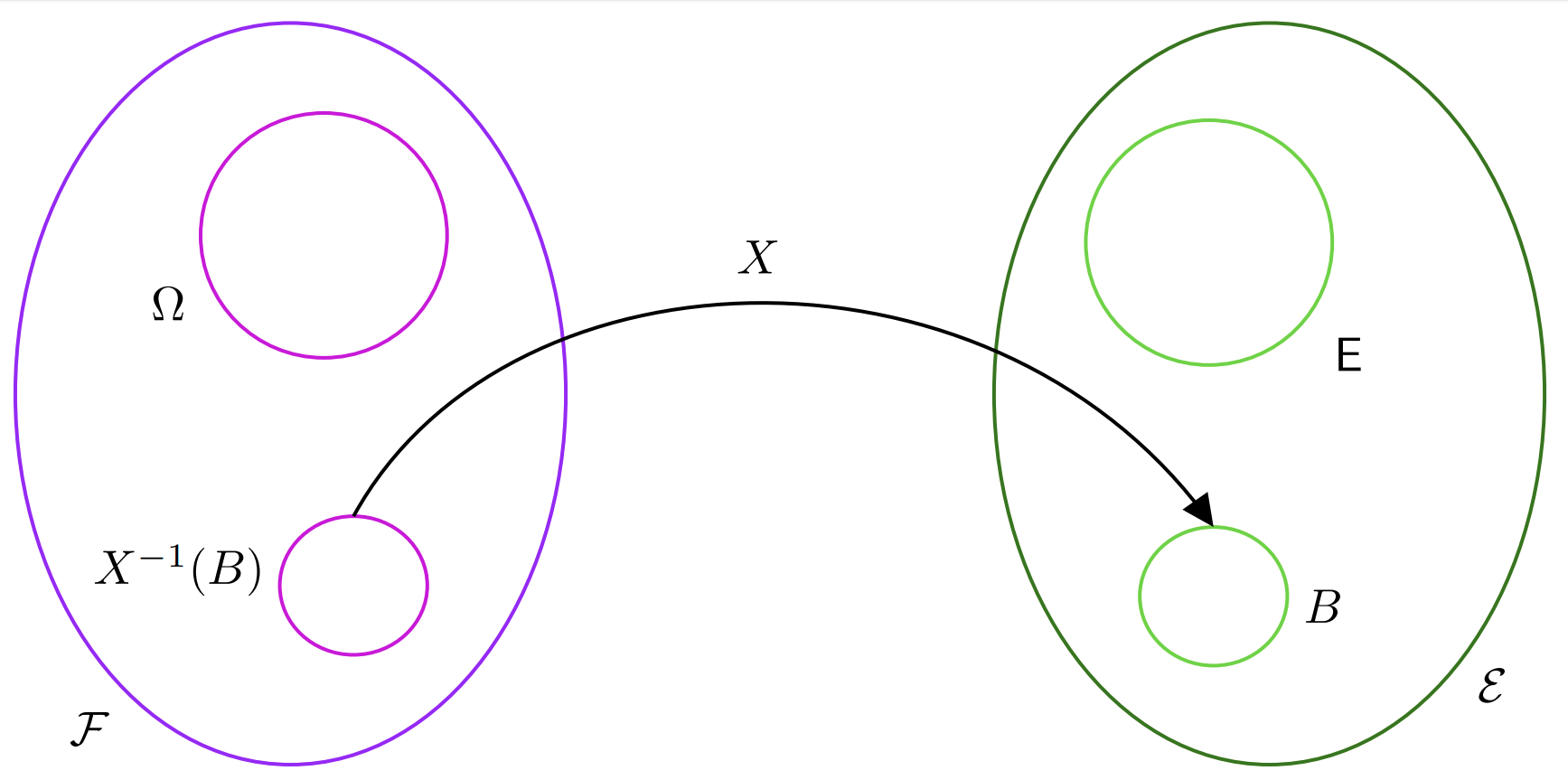
In the diagram above we can see how the set \(B\), which is an element of \(\mathcal{E}\) has a pre-image, which we call \(X^{-1}(B)\), which is an element of \(\mathcal{F}\)!

Probability Distribution

A probability distribution is also called a pushforward measure of the probability measure \(\mathbb{P}\) via the random variable \(X\). Suppose we have a probability space \((\Omega, \mathcal{F}, \mathbb{P})\). This means we can assign probabilities to events in \(\mathcal{F}\). Now suppose we have a measurable spae \((\mathsf{E}, \mathcal{E})\) but we don’t yet have a probability measure to measure events in it. How can we go about measuring sets in \(\mathcal{E}\)?

The key idea is that, given a set \(B\) in \(\mathcal{E}\), we can use a random variable \(X\) to find the pre-image of such set in the event space \(\mathcal{F}\) and then measure this set via the probability measure \(\mathcal{P}\). This will then be our probability measurament also for \(B\), as shown in the figure below.

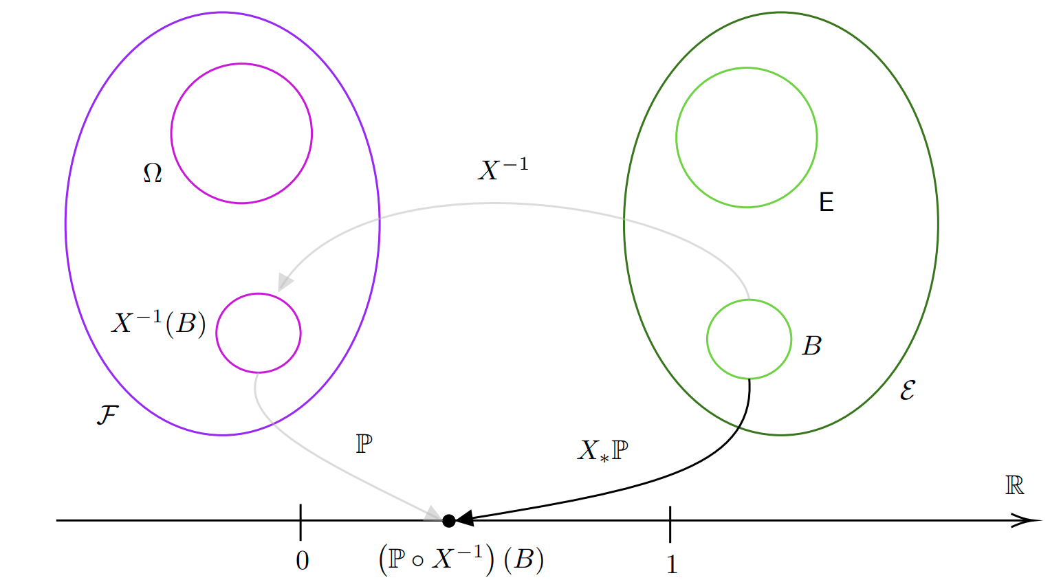
The probability distribution, or pushforward, is then denoted as \(X_*\mathbb{P}\) or \(\mathbb{P} \circ X^{-1}\). The probability distribution is therefore a function mapping sets in \(\mathcal{E}\) into \([0, 1]\): \[ X^*\mathbb{P}: \mathcal{E} \to [0, 1] \] In practice one often uses \((\mathsf{E}, \mathcal{E}) = (\mathbb{R}^n, \mathcal{B}(\mathbb{R}^n))\) so we have \[ X^*\mathbb{P}: \mathcal{B}(\mathbb{R}^n) \to [0, 1] \]

Probability Density Function

Consider \((\mathbb{R}^n, \mathcal{B}(\mathbb{R}^n))\). Suppose we have the usual Lebesgue measure \(\lambda^n\) on such a measurable space. This would assign to each set \(A\in\mathcal{B}(\mathbb{R}^n)\) our usual idea of size. However, now we have the random variable \(X\) and we would like to “weight” the size of a set \(A\in\mathcal{B}(\mathbb{R}^n)\) based on the “likelihood” of it happening. To do so, we assign a density to every point in \(\mathbb{R}^n\) and to compute the new measure of \(A\) according to \(X_*\mathbb{P}\) we simply take the average of its density at all points in \(A\) according to the Lebesgue measure \[ X_*\mathbb{P}(A) = \int_AdX_*\mathbb{P} = \int_A f d\lambda^n \qquad \forall A\in\mathcal{B}(\mathbb{R}^n) \] Essentially the density is almost like a derivative in the sense that it describes the rate of change of density of \(dX_*\mathbb{P}\) with respect to \(\lambda^n\). For this reason, we denote the density \(f\) as follows \[ f = \frac{d X_*\mathbb{P}}{d \lambda^n}. \] This is called the Radon-Nikodym derivative. Using this notation is very convenient because we can use it to change the measure we are using to integrate. \[ X_*\mathbb{P}(A) = \int_A d X_*\mathbb{P} = \int_A \frac{dX_*\mathbb{P}}{d \lambda^n} d\lambda^n = \int_Af d\lambda^n \] The function \(f\) is called the probability density function of the random variable \(X\). Notice how one can express the probability distribution also in terms of the original probability measure \[ p(A) = X_*\mathbb{P}(A) = \int_A d\mathbb{P}\circ X^{-1} = \int_{X^{-1}(A)}d \mathbb{P} \]

Expectation, Change of Variable and Law of the Unconscious Statistician

The expectation of the random variable \(X\) is given by the following Lebesgue integral \[ \mathbb{E}_{\mathbb{P}}[X] = \int_{\Omega} X d\mathbb{P} = \int_{\Omega}X(\omega) d\mathbb{P}(\omega) \] There is an important theorem called change of variable formula (i.e. LOTUS) that tells us that we can write the expectation of a tranformed random variable \(g \circ X: \Omega \to \mathbb{R}^n\) where \(g:\mathbb{R}^n \to \mathbb{R}^n\) in terms of the Lebesgue measure as follows \[ \mathbb{E}_{\mathbb{P}}[g \circ X] = \int_{\Omega} g \circ X \, d\mathbb{P} = \int_{\mathbb{R}^n} g \, dX_*\mathbb{P} = \int_{\mathbb{R}^n} g \frac{d X_*\mathbb{P}}{d\lambda^n} d\lambda^n = \int_{\mathbb{R}^n}g f \, d\lambda^n = \int_{\mathbb{R}^n} g(x) f(x) dx \] Importantly notice how the initial integral as over \(\Omega\) and now it’s over \(X(\Omega) = \mathbb{R}^n\).

Markov Transition Kernel

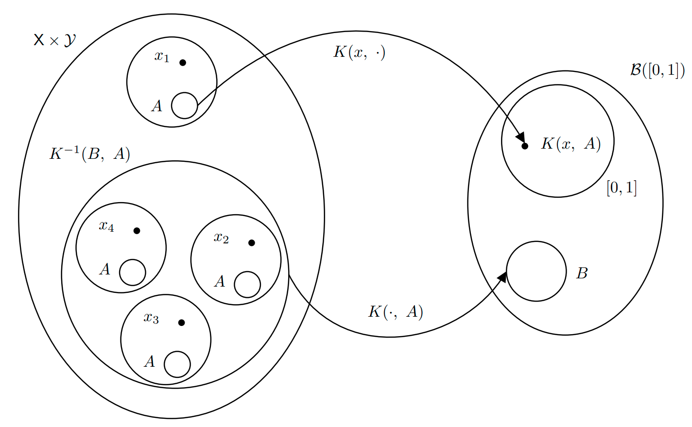
Let \((S, \mathcal{S})\) and \((T, \mathcal{T})\) be two measurable spaces. A Markov Kernel is a map \[ K: S \times \mathcal{T} \to [0, 1] \] satisfying the following properties:

• \(K(x, \cdot): \mathcal{T} \to [0, 1]\) is a probability measure for every \(x\in S\). In practice this means that \(K(x, \cdot)\) measures the probability of jumping from \(X\in S\) to any point \(y\in A\in \mathcal{T}\).
• \(K(\cdot, A): S\to [0,1]\) is a measurable function. This means that given a set \(A\) to jump to, the function that maps a point to the probability of jumping to any point in \(A\) is measurable, i.e. a random variable.

The Markov Kernel defines two operators:

• It operates on the left with measures: Let \(\mu\) be a measure on \((S, \mathcal{S})\). Then \(\mu K\) is a measure on \((T, \mathcal{T})\) \[ \mu K(A) = \int_S \mu(dx) K(x, A) \qquad \qquad A\in\mathcal{T} \] Basically \(\mu K\) gives you the average probability of jumping to some point \(y\in A\) where \(A\in\mathcal{T}\) if you start from point with measure \(\mu\). Indeed, if we define \(K_A: S \to [0, 1]\) as \(K_A(x) = K(x, A)\) then we can write \[ \mu K(A) = \mathbb{E}_\mu[K_A] = \int_S K_A d\mu = \int_S K_A(x) d\mu(x) = \int_S K(x, A) \mu(dx) \]

• It operates on the right with measurable functions

This is heavily influenced by https://www.randomservices.org/random/expect/Kernels.html.